Add a reference point approach for multi-objective optimization to a multi-objective conservation planning problem (Wierzbicki 1980, López Jaimes 2009). Broadly speaking, this approach considers a set of (i) reference point parameters that specify an aspirational level of achievement for each objective and (ii) weight parameters that specify the relative importance for reaching the reference point for each objective. To ensure that solutions are not biased by differences in scale among the objectives, this approach also considers the best and worst possible objective values for each objective.
Usage
add_ref_point_approach(
  x,
  weights = NULL,
  ref_points = NULL,
  best = NULL,
  worst = NULL,
  rescale = TRUE,
  verbose = TRUE
)
Arguments
- x
multi_problem()object.- weights
numericvector containing the weights for each objective. To generate multiple solutions based on different values,weightscan be anumericmatrix where each row corresponds to a different solution and each column corresponds to a different objective. Defaults toNULLsuch that weights are automatically calculated to equally balance all objectives (i.e., equivalent to anumericvector containing a value of 1 for each objective).- ref_points
numericvector containing values that denote the reference points. These points represent aspirational goals for each objective. To generate multiple solutions based on different values,ref_pointscan be anumericmatrix where each row corresponds to a different solution and each columns corresponds to a different objective. Note that all values must be greater than zero. Defaults toNULLsuch that reference points are automatically calculated based on the best possible objective value for each objective.- best
numericvector containing objective values that denote the best possible performance for each objective. Note that values must follow the same order as the problems inx. Defaults toNULLsuch that these values are computed automatically.- worst
numericvector containing objective values that denote the worst possible performance for each objective. Note that values must follow the same order as the problems inx. Defaults toNULLsuch that these values are computed automatically.- rescale
logicalindicating ifweightsshould be normalized based on the best and worst objective values (perbestandworst, respectively). This is important to ensure that the optimization process is not biased by differences in scale between different objectives. Defaults toTRUE.- verbose
logicalshould progress on generating multiple solutions be displayed? Defaults toTRUE.
Value
An updated multi_problem() object with the approach
added to it.
Details
The reference point approach for multi-objective optimization involves creating a new objective that is calculated based on multiple objectives. In particular, the new objective uses weights to specify the relative importance of each individual objective, and reference points to specify a desirable threshold level of performance for each objective (conceptually similar to target thresholds used in conservation planning). Given this, the reference point approach first involves calculate the weighted shortfall for each objective (i.e., difference between the reference point and the objective value for a candidate solution, multiplied by the weight). It then involves maximizing the maximum value of the weighted shortfalls, and then subsequently minimizing the sum of the weighted shortfalls.
To describe this approach mathematically, we will define the
following terminology.
Although this approach can support both maximization and minimization
objectives, we will assume that all objectives should
be maximized for brevity.
Let \(O\) denote the set of objectives (indexed by \(o\)).
For each objective, let \(w_o\) denote the weight for each objective
\(o \in O\) (per weights),
\(r_o\) denote the reference point for each objective
\(o \in O\) (per ref_points),
\(b_o\) denote the best objective value for each objective
(per best),
\(c_o\) denote the worst objective value for each objective
(per worst),
\(s_o\) denote a scaling term for each objective
(see below for details),
and \(v_o\) denote the objective value
for a candidate solution as measured based on each objective
\(o \in O\).
After defining these terms, the approach
is formulated with the following equation.
$$ \mathrm{Minimize} \space \max_{o \in O} w_o \times s_o \times \max(r_o - v_o, 0), \\ \mathrm{Minimize} \space \sum_{o \in O} w_o \times s_o \times \max(r_o - v_o, 0) $$
If the weights should be normalized (per rescale = TRUE), then
the scaling term for each objective is calculated
with the following equation.
$$ so = \frac{1}{\|bo - co\|} $$
Conversely, if the weights should not be normalized
(per rescale = FALSE), then \(s_o\)
is set to a value of 1 for each objective.
References
López Jaimes A, Zapotecas Martínez S, and Coello Coello CA (2009) An introduction to multiobjective optimization techniques in Optimization in Polymer Processing. Eds Gaspar-Cunha A and Covas JA. Nova Science Publishers Inc, New York, United States.
Wierzbicki AP (1980) The use of reference objectives in multiobjective optimization in Multiple criteria decision making theory and application. Eds Fandel G and Gal T. Lecture notes in economics and mathematical systems (pp. 468–486). Springer Berlin Heidelberg.
See also
Other functions for adding multi-objective optimization approaches:
add_hier_approach(),
add_wtd_sum_approach()
Examples
# in this example, we aim to identify a set of planning units that will
# not exceed a particular budget and meet objectives for
# (i) representing species that are important for ecosystem
# functioning (hereafter, keystone species) and (ii) representing species
# that have high social or cultural value (hereafter, iconic species)
# import data
con_cost <- get_sim_pu_raster()
keystone_spp <- get_sim_features()[[1:3]]
iconic_spp <- get_sim_features()[[4:5]]
# define a total conservation budget (30% of total cost)
budget <- terra::global(con_cost, "sum", na.rm = TRUE)[[1]] * 0.3
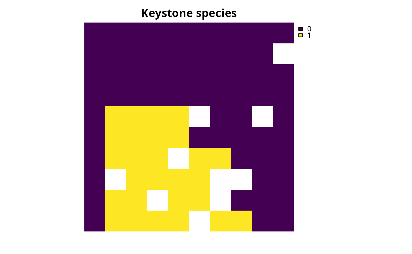
# define a single-objective problem for the keystone species objective
p1 <-
problem(con_cost, keystone_spp) %>%
add_min_shortfall_objective(budget) %>%
add_relative_targets(0.4) %>%
add_binary_decisions()
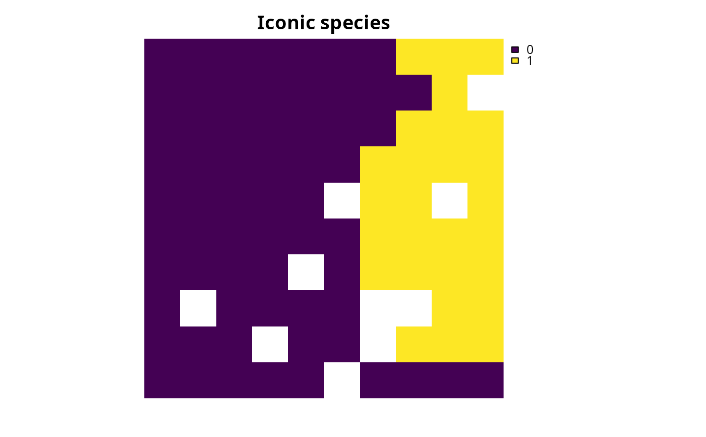
# define a single-objective problem for the iconic species objective
p2 <-
problem(con_cost, iconic_spp) %>%
add_min_shortfall_objective(budget) %>%
add_relative_targets(0.45) %>%
add_binary_decisions()
# solve the single-objective problems
s1 <-
p1 %>%
add_default_solver(verbose = FALSE) %>%
solve()
s2 <-
p2 %>%
add_default_solver(verbose = FALSE) %>%
solve()
# plot the solutions to the single-objective problems
plot(s1, main = "Keystone species", axes = FALSE)
 plot(s2, main = "Iconic species", axes = FALSE)
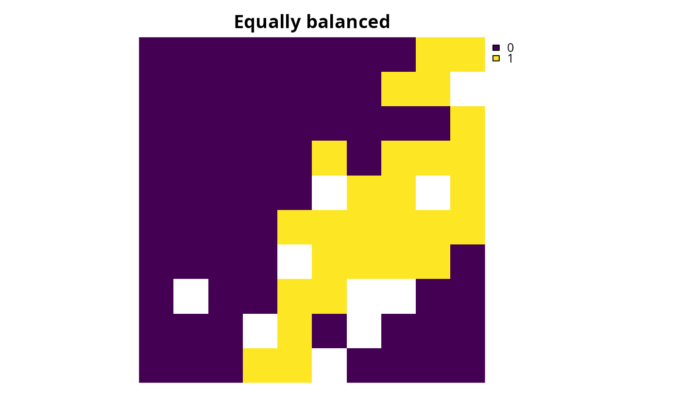
 # now create multi-objective problem with reference point approach,
# with settings to automatically identify an equally balanced solution
mp1 <-
multi_problem(keystone_obj = p1, iconic_obj = p2) %>%
add_ref_point_approach(verbose = TRUE) %>%
add_default_solver(verbose = FALSE)
# solve problem
ms1 <- solve(mp1)
# plot solution to multi-objective problem
plot(ms1, main = "Equally balanced", axes = FALSE)
# now create multi-objective problem with reference point approach,
# with settings to automatically identify an equally balanced solution
mp1 <-
multi_problem(keystone_obj = p1, iconic_obj = p2) %>%
add_ref_point_approach(verbose = TRUE) %>%
add_default_solver(verbose = FALSE)
# solve problem
ms1 <- solve(mp1)
# plot solution to multi-objective problem
plot(ms1, main = "Equally balanced", axes = FALSE)
 # we will now generate multiple solutions based on a matrix
# that contains different combinations of weight values
# create a matrix with weight values for objectives
weights_matrix <- approach_weights_matrix(
n_problems = 2, n_values = 5, include_zero = TRUE
)
# print weight matrix
print(weights_matrix)
#> [,1] [,2]
#> [1,] 1.00 1.00
#> [2,] 1.00 0.00
#> [3,] 0.00 1.00
#> [4,] 0.50 0.25
#> [5,] 0.75 0.25
#> [6,] 1.00 0.25
#> [7,] 0.25 0.50
#> [8,] 0.75 0.50
#> [9,] 1.00 0.50
#> [10,] 0.25 0.75
#> [11,] 0.50 0.75
#> [12,] 1.00 0.75
#> [13,] 0.25 1.00
#> [14,] 0.50 1.00
#> [15,] 0.75 1.00
# now create multi-objective problem with reference point approach,
# with weights to generate multiple solutions
mp2 <-
multi_problem(keystone_obj = p1, iconic_obj = p2) %>%
add_ref_point_approach(weights = weights_matrix, verbose = TRUE) %>%
add_default_solver(gap = 0.01, verbose = FALSE)
# solve multi-objective problem and remove duplicate solutions
ms2 <- solve(mp2, remove_duplicates = TRUE)
#> Generating solutions ■■■■■■■ | 3/15 | 20% | ETA: 5s
#> Generating solutions ■■■■■■■■■■■■■■■■■■■ | 9/15 | 60% | ETA: 3s
#> Generating solutions ■■■■■■■■■■■■■■■■■■■■■■■■■■■■■■■ | 15/15 | 100% | ETA: 0s
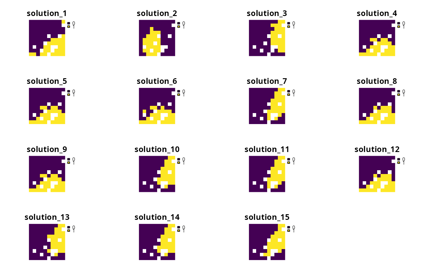
# plot multiple solutions
plot(terra::rast(ms2), axes = FALSE)
# we will now generate multiple solutions based on a matrix
# that contains different combinations of weight values
# create a matrix with weight values for objectives
weights_matrix <- approach_weights_matrix(
n_problems = 2, n_values = 5, include_zero = TRUE
)
# print weight matrix
print(weights_matrix)
#> [,1] [,2]
#> [1,] 1.00 1.00
#> [2,] 1.00 0.00
#> [3,] 0.00 1.00
#> [4,] 0.50 0.25
#> [5,] 0.75 0.25
#> [6,] 1.00 0.25
#> [7,] 0.25 0.50
#> [8,] 0.75 0.50
#> [9,] 1.00 0.50
#> [10,] 0.25 0.75
#> [11,] 0.50 0.75
#> [12,] 1.00 0.75
#> [13,] 0.25 1.00
#> [14,] 0.50 1.00
#> [15,] 0.75 1.00
# now create multi-objective problem with reference point approach,
# with weights to generate multiple solutions
mp2 <-
multi_problem(keystone_obj = p1, iconic_obj = p2) %>%
add_ref_point_approach(weights = weights_matrix, verbose = TRUE) %>%
add_default_solver(gap = 0.01, verbose = FALSE)
# solve multi-objective problem and remove duplicate solutions
ms2 <- solve(mp2, remove_duplicates = TRUE)
#> Generating solutions ■■■■■■■ | 3/15 | 20% | ETA: 5s
#> Generating solutions ■■■■■■■■■■■■■■■■■■■ | 9/15 | 60% | ETA: 3s
#> Generating solutions ■■■■■■■■■■■■■■■■■■■■■■■■■■■■■■■ | 15/15 | 100% | ETA: 0s
# plot multiple solutions
plot(terra::rast(ms2), axes = FALSE)
 # extract objective values for the solutions
obj_matrix <- attributes(ms2)$objective
# print the objective values
print(obj_matrix)
#> keystone_obj iconic_obj
#> solution_1 0.9616594 0.6677060
#> solution_2 0.8567573 2.0000000
#> solution_3 3.0000000 0.6033789
#> solution_4 0.8949350 0.7202442
#> solution_5 0.8949350 0.7202442
#> solution_6 0.8893569 0.7320958
#> solution_7 1.0622668 0.6105064
#> solution_8 0.9061754 0.7086196
#> solution_9 0.8949350 0.7202442
#> solution_10 1.0759486 0.6061551
#> solution_11 1.0622668 0.6105064
#> solution_12 0.9061754 0.7086196
#> solution_13 1.0776369 0.6058445
#> solution_14 1.0759486 0.6061551
#> solution_15 1.0485940 0.6175877
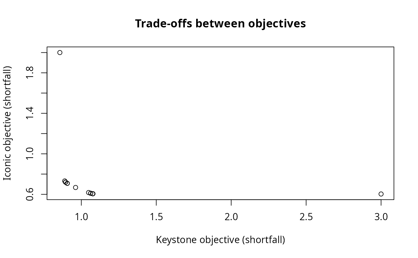
# plot the objectives values to visualize trade-offs
# (note that smaller values are better because these objectives seek to
# minimize representation shortfalls)
plot(
obj_matrix,
main = "Trade-offs between objectives",
xlab = "Keystone objective (shortfall)",
ylab = "Iconic objective (shortfall)"
)
# extract objective values for the solutions
obj_matrix <- attributes(ms2)$objective
# print the objective values
print(obj_matrix)
#> keystone_obj iconic_obj
#> solution_1 0.9616594 0.6677060
#> solution_2 0.8567573 2.0000000
#> solution_3 3.0000000 0.6033789
#> solution_4 0.8949350 0.7202442
#> solution_5 0.8949350 0.7202442
#> solution_6 0.8893569 0.7320958
#> solution_7 1.0622668 0.6105064
#> solution_8 0.9061754 0.7086196
#> solution_9 0.8949350 0.7202442
#> solution_10 1.0759486 0.6061551
#> solution_11 1.0622668 0.6105064
#> solution_12 0.9061754 0.7086196
#> solution_13 1.0776369 0.6058445
#> solution_14 1.0759486 0.6061551
#> solution_15 1.0485940 0.6175877
# plot the objectives values to visualize trade-offs
# (note that smaller values are better because these objectives seek to
# minimize representation shortfalls)
plot(
obj_matrix,
main = "Trade-offs between objectives",
xlab = "Keystone objective (shortfall)",
ylab = "Iconic objective (shortfall)"
)