Solve a conservation planning problem.
Usage
# S3 method for class 'ConservationProblem'
solve(a, b, ..., run_checks = TRUE, force = FALSE, remove_duplicates = FALSE)

# S3 method for class 'MultiConservationProblem'
solve(a, b, ..., run_checks = TRUE, force = FALSE, remove_duplicates = FALSE)
Arguments
- a
problem()ormulti_problem()object.- b
missing.
- ...
arguments passed to
compile().- run_checks
logicalvalue indicating if presolve checks should be run prior solving the problem. These checks are performed using thepresolve_check()function. Defaults toTRUE. Note that skipping these checks may reduce run time for large problems.- force
logicalvalue indicating if an attempt to should be made to solve the problem even if potential issues were detected during the presolve checks. Defaults toFALSE.- remove_duplicates
logicalvalue indicating if duplicated solutions should be removed. Note thatremove_duplicatesonly has an affect ifahas a portfolio or multi-objective optimization approach that involves generating multiple solutions (see portfolios and approaches for details). Defaults toFALSE.
Value
A numeric, matrix, data.frame, sf::st_sf(), or
terra::rast(), or list object containing the solution(s) to the problem.
Although solutions will generally be returned in the same format
as the planning units in a, these solutions may be returned in a list
object if multiple solutions are produced during the optimization process
(see Output format section for further details).
Details
After formulating a conservation planning problem(),
it can be solved using an exact algorithm solver (see solvers
for available solvers). If no solver has been explicitly specified,
then the best available exact algorithm solver will be used by default
(see add_default_solver()). Although these exact algorithm
solvers will often display a lot of information that isn't really that
helpful (e.g., nodes, cutting planes), they do display information
about the progress they are making on solving the problem (e.g., the
performance of the best solution found at a given point in time). If
potential issues were detected during the
presolve checks (see presolve_check())
and the problem is being forcibly solved (i.e., with force = TRUE),
then it is also worth checking for any warnings displayed by the solver
to see if these potential issues are actually causing issues
(e.g., Gurobi can display warnings that include
"Warning: Model contains large matrix coefficient range" and
"Warning: Model contains large rhs").
Output format
This function will output solutions in a similar format to the
planning units associated with a. Note that if multiple solutions are
generated (e.g., see portfolios and (see approaches),
then each solution may be returned as an element of a list object.
Specifically, the solutions will have the following format based on
the types of planning units in a.
ahasnumericplanning unitsHere the solution will be returned as a
numericvector. In particular, each element in the vector corresponds to a different planning unit. Note that if a portfolio is used to generate multiple solutions, then alistof suchnumericvectors will be returned.ahasmatrixplanning unitsHere the solution will be returned as a
matrixobject. In particular, rows correspond to different planning units, and columns correspond to different management zones. Note that if a portfolio is used to generate multiple solutions, then alistof suchmatrixobjects will be returned.ahasterra::rast()planning unitsHere the solution will be returned as a
terra::rast()object. Ifacontains multiple zones, then the solution object will have a different layer for each management zone. Note that if a portfolio is used to generate multiple solutions, then alistofterra::rast()objects will be returned.ahassf::sf(), ordata.frameplanning unitsHere the solution will be returned in the same data format as the planning units. In particular, each row corresponds to a different planning unit, and columns contain solutions. If
acontains a single zone, then the solution object will contain columns named by solution. Specifically, the column names containing the solution values be will named as"solution_XXX"where"XXX"corresponds to a solution identifier (e.g.,"solution_1"). Ifacontains multiple zones, then the columns containing solutions will be named as"solution_XXX_YYY"where"XXX"corresponds to the solution identifier and"YYY"is the name of the management zone (e.g.,"solution_1_zone1").
The output solutions have attributes that describe optimization process or solution (see below for examples on accessing these attributes). These attributes provide the following information.
objectivenumericmathematical objective value for the solution used to evaluate the prioritization during optimization.runtimenumerictotal amount of time elapsed while during the optimization process (reported in seconds). Note that this measure of time does not include any data pre-processing or post-processing steps.statuscharacterstatus of the optimization process. This status typically describes the reason why the optimization process terminated. For example, it might indicate that the optimization process terminated because an optimal solution was found, or because a pre-specified time limit was reached. These status values are (mostly) obtained directly from the solver software, and so we recommend consulting the solver's documentation for further information on what particular status values mean. Note that some solvers (e.g., Gurobi and HiGHS) will return an"OPTIMAL"status when the solver has found a solution within the pre-specified optimality gap (e.g., it has found a solution within 10% of optimality), even though the solution itself may not be strictly optimal.gapnumericoptimality of the solution. This gap value provides an upper bound of how far the solution is from optimality. For example, you might specify a 10% optimality gap for the optimization process (e.g., usingadd_highs_solver(gap = 0.1)), and this might produce a solution that is actually 5% from optimality. As such, the solution might have a gap value of 0.05 (corresponding to 5%). Because this value represents an upper bound, it is also possible that the solution in this example – even though it is actually 5% from optimality – might have a gap value of 7% (i.e., 0.07). Note that only some solvers are able to provide this information (i.e., the Gurobi and HiGHS solvers), and other solvers will have a missing (NA) value.objboundnumericbest known bound of the optimal objective. Note that only some solvers are able to provide this information (i.e., the Gurobi solvers), and other solvers will have a missing (NA) value.
See also
See problem() and multi_problem() to create conservation planning
problems. Also, see presolve_check() to check problems for potential
issues prior to solving a problem, and category_layer() and
category_vector() to reformat solutions that contain multiple zones.
Examples
# set seed for reproducibility
set.seed(500)
# load data
sim_pu_raster <- get_sim_pu_raster()
sim_pu_polygons <- get_sim_pu_polygons()
sim_features <- get_sim_features()
sim_zones_pu_raster <- get_sim_zones_pu_raster()
sim_zones_pu_polygons <- get_sim_zones_pu_polygons()
sim_zones_features <- get_sim_zones_features()
# build minimal conservation problem with raster data
p1 <-
problem(sim_pu_raster, sim_features) %>%
add_min_set_objective() %>%
add_relative_targets(0.1) %>%
add_binary_decisions() %>%
add_default_solver(verbose = FALSE)
# solve the problem
s1 <- solve(p1)
# print solution
print(s1)
#> class : SpatRaster
#> size : 10, 10, 1 (nrow, ncol, nlyr)
#> resolution : 0.1, 0.1 (x, y)
#> extent : 0, 1, 0, 1 (xmin, xmax, ymin, ymax)
#> coord. ref. : WGS 84 / Pseudo-Mercator (EPSG:3857)
#> source(s) : memory
#> varname : sim_pu_raster
#> name : layer
#> min value : 0
#> max value : 1
# print attributes describing the optimization process and the solution
print(attr(s1, "objective"))
#> solution_1
#> 1987.399
print(attr(s1, "runtime"))
#> solution_1
#> 0.005
print(attr(s1, "status"))
#> solution_1
#> "OPTIMAL"
print(attr(s1, "gap"))
#> solution_1
#> 0.02808527
# calculate feature representation in the solution
r1 <- eval_feature_representation_summary(p1, s1)
print(r1)
#> # A tibble: 5 × 5
#> summary feature total_amount absolute_held relative_held
#> <chr> <chr> <dbl> <dbl> <dbl>
#> 1 overall feature_1 83.3 8.91 0.107
#> 2 overall feature_2 31.2 3.13 0.100
#> 3 overall feature_3 72.0 7.34 0.102
#> 4 overall feature_4 42.7 4.35 0.102
#> 5 overall feature_5 56.7 6.01 0.106
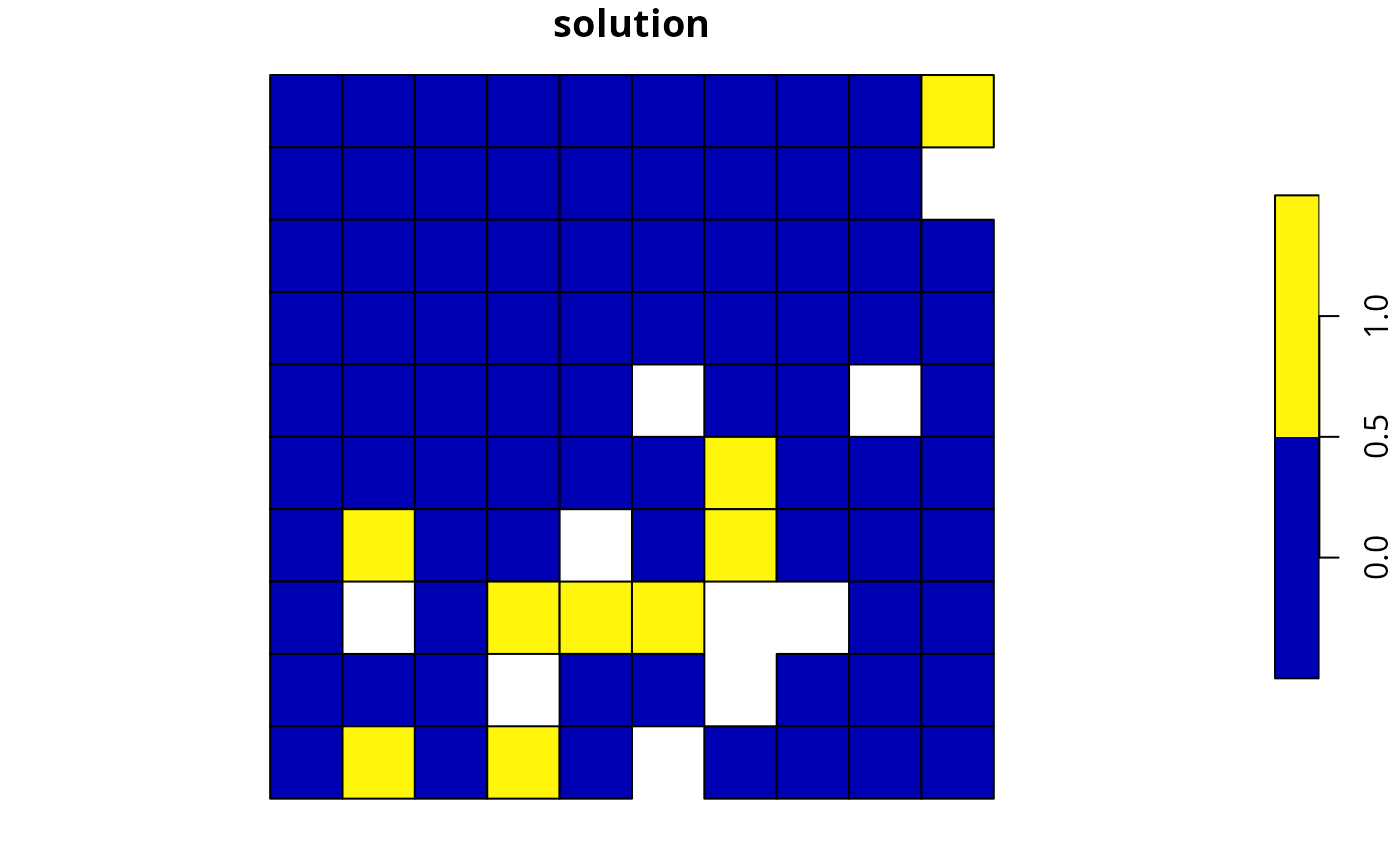
# plot solution
plot(s1, main = "solution", axes = FALSE)
 # build minimal conservation problem with polygon data
p2 <-
problem(sim_pu_polygons, sim_features, cost_column = "cost") %>%
add_min_set_objective() %>%
add_relative_targets(0.1) %>%
add_binary_decisions() %>%
add_default_solver(verbose = FALSE)
# solve the problem
s2 <- solve(p2)
# print solution
print(s2)
#> Simple feature collection with 90 features and 4 fields
#> Geometry type: POLYGON
#> Dimension: XY
#> Bounding box: xmin: 0 ymin: 0 xmax: 1 ymax: 1
#> Projected CRS: WGS 84 / Pseudo-Mercator
#> # A tibble: 90 × 5
#> cost locked_in locked_out solution_1 geometry
#> * <dbl> <lgl> <lgl> <dbl> <POLYGON [m]>
#> 1 216. FALSE FALSE 0 ((0 1, 0.1 1, 0.1 0.9, 0 0.9, 0 1))
#> 2 213. FALSE FALSE 0 ((0.1 1, 0.2 1, 0.2 0.9, 0.1 0.9, 0.1 …
#> 3 207. FALSE FALSE 0 ((0.2 1, 0.3 1, 0.3 0.9, 0.2 0.9, 0.2 …
#> 4 209. FALSE TRUE 0 ((0.3 1, 0.4 1, 0.4 0.9, 0.3 0.9, 0.3 …
#> 5 214. FALSE FALSE 0 ((0.4 1, 0.5 1, 0.5 0.9, 0.4 0.9, 0.4 …
#> 6 214. FALSE FALSE 0 ((0.5 1, 0.6 1, 0.6 0.9, 0.5 0.9, 0.5 …
#> 7 210. FALSE FALSE 0 ((0.6 1, 0.7 1, 0.7 0.9, 0.6 0.9, 0.6 …
#> 8 211. FALSE TRUE 0 ((0.7 1, 0.8 1, 0.8 0.9, 0.7 0.9, 0.7 …
#> 9 210. FALSE FALSE 0 ((0.8 1, 0.9 1, 0.9 0.9, 0.8 0.9, 0.8 …
#> 10 204. FALSE FALSE 0 ((0.9 1, 1 1, 1 0.9, 0.9 0.9, 0.9 1))
#> # ℹ 80 more rows
# calculate feature representation in the solution
r2 <- eval_feature_representation_summary(p2, s2[, "solution_1"])
print(r2)
#> # A tibble: 5 × 5
#> summary feature total_amount absolute_held relative_held
#> <chr> <chr> <dbl> <dbl> <dbl>
#> 1 overall feature_1 74.5 8.05 0.108
#> 2 overall feature_2 28.1 2.83 0.101
#> 3 overall feature_3 64.9 6.65 0.103
#> 4 overall feature_4 38.2 3.87 0.101
#> 5 overall feature_5 50.7 5.41 0.107
# plot solution
plot(s2[, "solution_1"], main = "solution", axes = FALSE)
# build minimal conservation problem with polygon data
p2 <-
problem(sim_pu_polygons, sim_features, cost_column = "cost") %>%
add_min_set_objective() %>%
add_relative_targets(0.1) %>%
add_binary_decisions() %>%
add_default_solver(verbose = FALSE)
# solve the problem
s2 <- solve(p2)
# print solution
print(s2)
#> Simple feature collection with 90 features and 4 fields
#> Geometry type: POLYGON
#> Dimension: XY
#> Bounding box: xmin: 0 ymin: 0 xmax: 1 ymax: 1
#> Projected CRS: WGS 84 / Pseudo-Mercator
#> # A tibble: 90 × 5
#> cost locked_in locked_out solution_1 geometry
#> * <dbl> <lgl> <lgl> <dbl> <POLYGON [m]>
#> 1 216. FALSE FALSE 0 ((0 1, 0.1 1, 0.1 0.9, 0 0.9, 0 1))
#> 2 213. FALSE FALSE 0 ((0.1 1, 0.2 1, 0.2 0.9, 0.1 0.9, 0.1 …
#> 3 207. FALSE FALSE 0 ((0.2 1, 0.3 1, 0.3 0.9, 0.2 0.9, 0.2 …
#> 4 209. FALSE TRUE 0 ((0.3 1, 0.4 1, 0.4 0.9, 0.3 0.9, 0.3 …
#> 5 214. FALSE FALSE 0 ((0.4 1, 0.5 1, 0.5 0.9, 0.4 0.9, 0.4 …
#> 6 214. FALSE FALSE 0 ((0.5 1, 0.6 1, 0.6 0.9, 0.5 0.9, 0.5 …
#> 7 210. FALSE FALSE 0 ((0.6 1, 0.7 1, 0.7 0.9, 0.6 0.9, 0.6 …
#> 8 211. FALSE TRUE 0 ((0.7 1, 0.8 1, 0.8 0.9, 0.7 0.9, 0.7 …
#> 9 210. FALSE FALSE 0 ((0.8 1, 0.9 1, 0.9 0.9, 0.8 0.9, 0.8 …
#> 10 204. FALSE FALSE 0 ((0.9 1, 1 1, 1 0.9, 0.9 0.9, 0.9 1))
#> # ℹ 80 more rows
# calculate feature representation in the solution
r2 <- eval_feature_representation_summary(p2, s2[, "solution_1"])
print(r2)
#> # A tibble: 5 × 5
#> summary feature total_amount absolute_held relative_held
#> <chr> <chr> <dbl> <dbl> <dbl>
#> 1 overall feature_1 74.5 8.05 0.108
#> 2 overall feature_2 28.1 2.83 0.101
#> 3 overall feature_3 64.9 6.65 0.103
#> 4 overall feature_4 38.2 3.87 0.101
#> 5 overall feature_5 50.7 5.41 0.107
# plot solution
plot(s2[, "solution_1"], main = "solution", axes = FALSE)
 # build multi-zone conservation problem with raster data
p3 <-
problem(sim_zones_pu_raster, sim_zones_features) %>%
add_min_set_objective() %>%
add_relative_targets(matrix(runif(15, 0.1, 0.2), nrow = 5, ncol = 3)) %>%
add_binary_decisions() %>%
add_default_solver(verbose = FALSE)
# solve the problem
s3 <- solve(p3)
# print solution
print(s3)
#> class : SpatRaster
#> size : 10, 10, 3 (nrow, ncol, nlyr)
#> resolution : 0.1, 0.1 (x, y)
#> extent : 0, 1, 0, 1 (xmin, xmax, ymin, ymax)
#> coord. ref. : WGS 84 / Pseudo-Mercator (EPSG:3857)
#> source(s) : memory
#> varnames : sim_zones_pu_raster
#> sim_zones_pu_raster
#> sim_zones_pu_raster
#> names : zone_1, zone_2, zone_3
#> min values : 0, 0, 0
#> max values : 1, 1, 1
# calculate feature representation in the solution
r3 <- eval_feature_representation_summary(p3, s3)
print(r3)
#> # A tibble: 20 × 5
#> summary feature total_amount absolute_held relative_held
#> <chr> <chr> <dbl> <dbl> <dbl>
#> 1 overall feature_1 250. 46.6 0.186
#> 2 overall feature_2 93.6 17.7 0.189
#> 3 overall feature_3 216. 41.6 0.193
#> 4 overall feature_4 128. 22.2 0.174
#> 5 overall feature_5 170. 30.7 0.180
#> 6 zone_1 feature_1 83.3 16.0 0.193
#> 7 zone_1 feature_2 31.2 5.47 0.175
#> 8 zone_1 feature_3 72.0 14.4 0.200
#> 9 zone_1 feature_4 42.7 6.41 0.150
#> 10 zone_1 feature_5 56.7 10.4 0.184
#> 11 zone_2 feature_1 83.3 16.0 0.192
#> 12 zone_2 feature_2 31.2 6.18 0.198
#> 13 zone_2 feature_3 72.0 14.5 0.201
#> 14 zone_2 feature_4 42.7 8.38 0.196
#> 15 zone_2 feature_5 56.7 10.3 0.181
#> 16 zone_3 feature_1 83.3 14.6 0.175
#> 17 zone_3 feature_2 31.2 6.01 0.193
#> 18 zone_3 feature_3 72.0 12.8 0.178
#> 19 zone_3 feature_4 42.7 7.42 0.174
#> 20 zone_3 feature_5 56.7 9.94 0.175
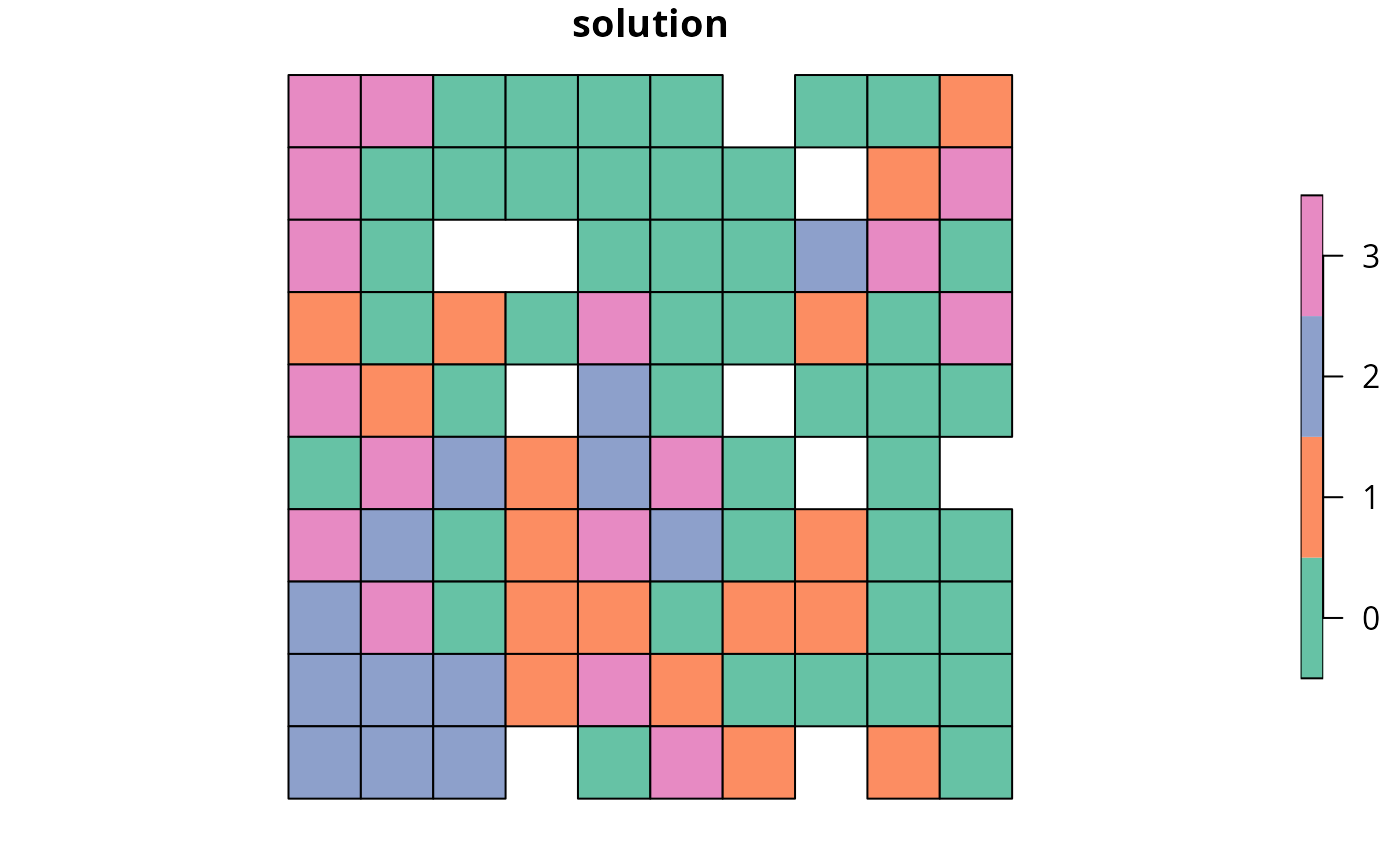
# plot solution
plot(category_layer(s3), main = "solution", axes = FALSE)
# build multi-zone conservation problem with raster data
p3 <-
problem(sim_zones_pu_raster, sim_zones_features) %>%
add_min_set_objective() %>%
add_relative_targets(matrix(runif(15, 0.1, 0.2), nrow = 5, ncol = 3)) %>%
add_binary_decisions() %>%
add_default_solver(verbose = FALSE)
# solve the problem
s3 <- solve(p3)
# print solution
print(s3)
#> class : SpatRaster
#> size : 10, 10, 3 (nrow, ncol, nlyr)
#> resolution : 0.1, 0.1 (x, y)
#> extent : 0, 1, 0, 1 (xmin, xmax, ymin, ymax)
#> coord. ref. : WGS 84 / Pseudo-Mercator (EPSG:3857)
#> source(s) : memory
#> varnames : sim_zones_pu_raster
#> sim_zones_pu_raster
#> sim_zones_pu_raster
#> names : zone_1, zone_2, zone_3
#> min values : 0, 0, 0
#> max values : 1, 1, 1
# calculate feature representation in the solution
r3 <- eval_feature_representation_summary(p3, s3)
print(r3)
#> # A tibble: 20 × 5
#> summary feature total_amount absolute_held relative_held
#> <chr> <chr> <dbl> <dbl> <dbl>
#> 1 overall feature_1 250. 46.6 0.186
#> 2 overall feature_2 93.6 17.7 0.189
#> 3 overall feature_3 216. 41.6 0.193
#> 4 overall feature_4 128. 22.2 0.174
#> 5 overall feature_5 170. 30.7 0.180
#> 6 zone_1 feature_1 83.3 16.0 0.193
#> 7 zone_1 feature_2 31.2 5.47 0.175
#> 8 zone_1 feature_3 72.0 14.4 0.200
#> 9 zone_1 feature_4 42.7 6.41 0.150
#> 10 zone_1 feature_5 56.7 10.4 0.184
#> 11 zone_2 feature_1 83.3 16.0 0.192
#> 12 zone_2 feature_2 31.2 6.18 0.198
#> 13 zone_2 feature_3 72.0 14.5 0.201
#> 14 zone_2 feature_4 42.7 8.38 0.196
#> 15 zone_2 feature_5 56.7 10.3 0.181
#> 16 zone_3 feature_1 83.3 14.6 0.175
#> 17 zone_3 feature_2 31.2 6.01 0.193
#> 18 zone_3 feature_3 72.0 12.8 0.178
#> 19 zone_3 feature_4 42.7 7.42 0.174
#> 20 zone_3 feature_5 56.7 9.94 0.175
# plot solution
plot(category_layer(s3), main = "solution", axes = FALSE)
 # build multi-zone conservation problem with polygon data
p4 <-
problem(
sim_zones_pu_polygons, sim_zones_features,
cost_column = c("cost_1", "cost_2", "cost_3")
) %>%
add_min_set_objective() %>%
add_relative_targets(matrix(runif(15, 0.1, 0.2), nrow = 5, ncol = 3)) %>%
add_binary_decisions() %>%
add_default_solver(verbose = FALSE)
# solve the problem
s4 <- solve(p4)
# print solution
print(s4)
#> Simple feature collection with 90 features and 9 fields
#> Geometry type: POLYGON
#> Dimension: XY
#> Bounding box: xmin: 0 ymin: 0 xmax: 1 ymax: 1
#> Projected CRS: WGS 84 / Pseudo-Mercator
#> # A tibble: 90 × 10
#> cost_1 cost_2 cost_3 locked_1 locked_2 locked_3 solution_1_zone_1
#> * <dbl> <dbl> <dbl> <lgl> <lgl> <lgl> <dbl>
#> 1 216. 183. 205. FALSE FALSE FALSE 0
#> 2 213. 189. 210. FALSE FALSE FALSE 0
#> 3 207. 194. 215. TRUE FALSE FALSE 0
#> 4 209. 198. 219. FALSE FALSE FALSE 0
#> 5 214. 200. 221. FALSE FALSE FALSE 0
#> 6 214. 203. 225. FALSE FALSE FALSE 0
#> 7 211. 209. 223. FALSE FALSE FALSE 0
#> 8 210. 212. 222. TRUE FALSE FALSE 0
#> 9 204. 218. 214. FALSE FALSE FALSE 0
#> 10 213. 183. 206. FALSE FALSE FALSE 0
#> # ℹ 80 more rows
#> # ℹ 3 more variables: solution_1_zone_2 <dbl>, solution_1_zone_3 <dbl>,
#> # geometry <POLYGON [m]>
# calculate feature representation in the solution
r4 <- eval_feature_representation_summary(
p4, s4[, c("solution_1_zone_1", "solution_1_zone_2", "solution_1_zone_3")]
)
print(r4)
#> # A tibble: 20 × 5
#> summary feature total_amount absolute_held relative_held
#> <chr> <chr> <dbl> <dbl> <dbl>
#> 1 overall feature_1 225. 37.7 0.167
#> 2 overall feature_2 83.9 14.8 0.177
#> 3 overall feature_3 195. 33.3 0.171
#> 4 overall feature_4 114. 19.2 0.168
#> 5 overall feature_5 154. 25.0 0.163
#> 6 zone_1 feature_1 75.1 12.3 0.164
#> 7 zone_1 feature_2 28.0 4.47 0.160
#> 8 zone_1 feature_3 65.0 10.7 0.164
#> 9 zone_1 feature_4 38.0 6.20 0.163
#> 10 zone_1 feature_5 51.2 8.06 0.158
#> 11 zone_2 feature_1 75.1 11.3 0.150
#> 12 zone_2 feature_2 28.0 5.28 0.189
#> 13 zone_2 feature_3 65.0 10.1 0.156
#> 14 zone_2 feature_4 38.0 6.85 0.180
#> 15 zone_2 feature_5 51.2 7.77 0.152
#> 16 zone_3 feature_1 75.1 14.1 0.188
#> 17 zone_3 feature_2 28.0 5.07 0.181
#> 18 zone_3 feature_3 65.0 12.5 0.193
#> 19 zone_3 feature_4 38.0 6.12 0.161
#> 20 zone_3 feature_5 51.2 9.16 0.179
# create new column representing the zone id that each planning unit
# was allocated to in the solution
s4$solution <- category_vector(
s4[, c("solution_1_zone_1", "solution_1_zone_2", "solution_1_zone_3")]
)
s4$solution <- factor(s4$solution)
# plot solution
plot(s4[, "solution"])
# build multi-zone conservation problem with polygon data
p4 <-
problem(
sim_zones_pu_polygons, sim_zones_features,
cost_column = c("cost_1", "cost_2", "cost_3")
) %>%
add_min_set_objective() %>%
add_relative_targets(matrix(runif(15, 0.1, 0.2), nrow = 5, ncol = 3)) %>%
add_binary_decisions() %>%
add_default_solver(verbose = FALSE)
# solve the problem
s4 <- solve(p4)
# print solution
print(s4)
#> Simple feature collection with 90 features and 9 fields
#> Geometry type: POLYGON
#> Dimension: XY
#> Bounding box: xmin: 0 ymin: 0 xmax: 1 ymax: 1
#> Projected CRS: WGS 84 / Pseudo-Mercator
#> # A tibble: 90 × 10
#> cost_1 cost_2 cost_3 locked_1 locked_2 locked_3 solution_1_zone_1
#> * <dbl> <dbl> <dbl> <lgl> <lgl> <lgl> <dbl>
#> 1 216. 183. 205. FALSE FALSE FALSE 0
#> 2 213. 189. 210. FALSE FALSE FALSE 0
#> 3 207. 194. 215. TRUE FALSE FALSE 0
#> 4 209. 198. 219. FALSE FALSE FALSE 0
#> 5 214. 200. 221. FALSE FALSE FALSE 0
#> 6 214. 203. 225. FALSE FALSE FALSE 0
#> 7 211. 209. 223. FALSE FALSE FALSE 0
#> 8 210. 212. 222. TRUE FALSE FALSE 0
#> 9 204. 218. 214. FALSE FALSE FALSE 0
#> 10 213. 183. 206. FALSE FALSE FALSE 0
#> # ℹ 80 more rows
#> # ℹ 3 more variables: solution_1_zone_2 <dbl>, solution_1_zone_3 <dbl>,
#> # geometry <POLYGON [m]>
# calculate feature representation in the solution
r4 <- eval_feature_representation_summary(
p4, s4[, c("solution_1_zone_1", "solution_1_zone_2", "solution_1_zone_3")]
)
print(r4)
#> # A tibble: 20 × 5
#> summary feature total_amount absolute_held relative_held
#> <chr> <chr> <dbl> <dbl> <dbl>
#> 1 overall feature_1 225. 37.7 0.167
#> 2 overall feature_2 83.9 14.8 0.177
#> 3 overall feature_3 195. 33.3 0.171
#> 4 overall feature_4 114. 19.2 0.168
#> 5 overall feature_5 154. 25.0 0.163
#> 6 zone_1 feature_1 75.1 12.3 0.164
#> 7 zone_1 feature_2 28.0 4.47 0.160
#> 8 zone_1 feature_3 65.0 10.7 0.164
#> 9 zone_1 feature_4 38.0 6.20 0.163
#> 10 zone_1 feature_5 51.2 8.06 0.158
#> 11 zone_2 feature_1 75.1 11.3 0.150
#> 12 zone_2 feature_2 28.0 5.28 0.189
#> 13 zone_2 feature_3 65.0 10.1 0.156
#> 14 zone_2 feature_4 38.0 6.85 0.180
#> 15 zone_2 feature_5 51.2 7.77 0.152
#> 16 zone_3 feature_1 75.1 14.1 0.188
#> 17 zone_3 feature_2 28.0 5.07 0.181
#> 18 zone_3 feature_3 65.0 12.5 0.193
#> 19 zone_3 feature_4 38.0 6.12 0.161
#> 20 zone_3 feature_5 51.2 9.16 0.179
# create new column representing the zone id that each planning unit
# was allocated to in the solution
s4$solution <- category_vector(
s4[, c("solution_1_zone_1", "solution_1_zone_2", "solution_1_zone_3")]
)
s4$solution <- factor(s4$solution)
# plot solution
plot(s4[, "solution"])