Getting started

Introduction

The aim of this tutorial is to provide a short introduction to the prioritizr R package. It is also intended to help conservation planners familiar the Marxan decision support tool (Ball et al. 2009) start using the package for their work.

Data

Let’s load the packages and data used in this tutorial. Since this tutorial uses data from the prioritizrdata R package, please ensure that it is installed. The data used in this tutorial were obtained from the Introduction to Marxan course and the Australian Government’s National Vegetation Information System.

# load packages
library(prioritizrdata)
library(prioritizr)
library(sf)
library(terra)
library(vegan)
library(cluster)

# set seed for reproducibility
set.seed(500)

# load planning unit data
tas_pu <- get_tas_pu()

# load feature data
tas_features <- get_tas_features()

Let’s have a look at the planning unit data. The tas_pu object contains planning units represented as spatial polygons (i.e., a sf::st_sf() object). This object has three columns that denote the following information for each planning unit: a unique identifier (id), unimproved land value (cost), and current conservation status (locked_in). Planning units that have at least half of their area overlapping with existing protected areas are denoted with a locked in TRUE value, otherwise they are denoted with a value of FALSE. We will also set the costs for existing protected areas to zero, so that existing protected areas aren’t included in the the cost of the prioritization.

# print planning unit data
print(tas_pu)

## Simple feature collection with 1130 features and 4 fields
## Geometry type: MULTIPOLYGON
## Dimension:     XY
## Bounding box:  xmin: 298809.6 ymin: 5167775 xmax: 613818.8 ymax: 5502544
## Projected CRS: WGS 84 / UTM zone 55S
## # A tibble: 1,130 × 5
##       id  cost locked_in locked_out                                         geom
##    <int> <dbl> <lgl>     <lgl>                                <MULTIPOLYGON [m]>
##  1     1 60.2  FALSE     TRUE       (((328497 5497704, 326783.8 5500050, 326775…
##  2     2 19.9  FALSE     FALSE      (((307121.6 5490487, 305344.4 5492917, 3053…
##  3     3 59.7  FALSE     TRUE       (((321726.1 5492382, 320111 5494593, 320127…
##  4     4 32.4  FALSE     FALSE      (((304314.5 5494324, 304342.2 5494287, 3043…
##  5     5 26.2  FALSE     FALSE      (((314958.5 5487057, 312336 5490646, 312339…
##  6     6 51.3  FALSE     FALSE      (((327904.3 5491218, 326594.6 5493012, 3284…
##  7     7 32.3  FALSE     FALSE      (((308194.1 5481729, 306601.2 5483908, 3066…
##  8     8 38.4  FALSE     FALSE      (((322792.7 5483624, 319965.3 5487497, 3199…
##  9     9  3.55 FALSE     FALSE      (((334896.6 5490731, 335610.4 5492490, 3357…
## 10    10  1.83 FALSE     FALSE      (((356377.1 5487952, 353903.1 5487635, 3538…
## # ℹ 1,120 more rows

# set costs for existing protected areas to zero
tas_pu$cost <- tas_pu$cost * !tas_pu$locked_in

# plot map of planning unit costs
plot(st_as_sf(tas_pu[, "cost"]), main = "Planning unit costs")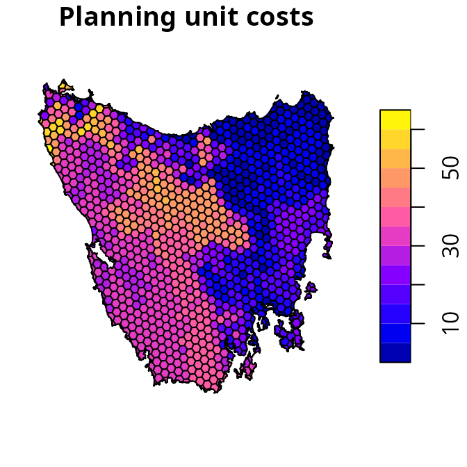

# plot map of planning unit coverage by protected areas
plot(st_as_sf(tas_pu[, "locked_in"]), main = "Protected area coverage")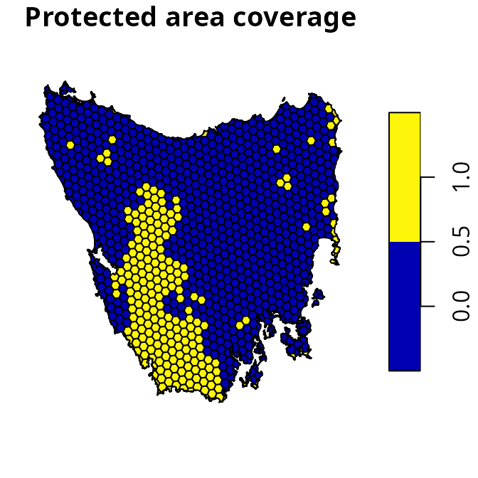

Now, let’s look at the conservation feature data. The tas_features object describes the spatial distribution of the features. Specifically, the feature data are a multi-layer raster (i.e., a terra::rast() object). Each layer corresponds to a different vegetation community. Within each layer, cells values denote the presence (using value of 1) or absence (using value of 0) of the vegetation community across the study area.

# print planning unit data
print(tas_features)

## class       : SpatRaster 
## size        : 398, 359, 33  (nrow, ncol, nlyr)
## resolution  : 1000, 1000  (x, y)
## extent      : 288801.7, 647801.7, 5142976, 5540976  (xmin, xmax, ymin, ymax)
## coord. ref. : WGS 84 / UTM zone 55S (EPSG:32755) 
## source      : tas_features.tif 
## names       : Banks~lands, Bould~marks, Calli~lands, Cool ~orest, Eucal~hyll), Eucal~torey, ... 
## min values  :           0,           0,           0,           0,           0,           0, ... 
## max values  :           1,           1,           1,           1,           1,           1, ...

# plot map of the first four vegetation classes
plot(tas_features[[1:4]])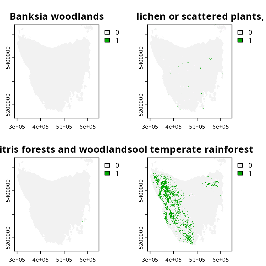

Problem formulation

Now we will formulate a conservation planing problem. To achieve this, we first specify which objects contain the planning unit and feature data (using the problem() function). Next, we specify that we want to use the minimum set objective function (using the add_min_set_objective() function). This objective function indicates that we wish to minimize the total cost of planning units selected by the prioritization. We then specify boundary penalties to reduce spatial fragmentation in the resulting prioritization (using the add_boundary_penalties() function; see the Calibrating trade-offs vignette for details on calibrating the penalty value). We also specify representation targets to ensure the resulting prioritization provides adequate coverage of each vegetation community (using the add_relative_targets() function). Specifically, we specify targets to ensure at least 17% of the spatial extent of each vegetation community (based on the Aichi Target 11). Additionally, we set constraints to ensure that planning units predominately covered by existing protected areas are selected by the prioritization (using the add_locked_in_constraints() function). Finally, we specify that the prioritization should either select – or not select – planning units for prioritization (using the add_binary_decisions() function).

# build problem
p1 <-
  problem(tas_pu, tas_features, cost_column = "cost") %>%
  add_min_set_objective() %>%
  add_boundary_penalties(penalty = 0.005) %>%
  add_relative_targets(0.17) %>%
  add_locked_in_constraints("locked_in") %>%
  add_binary_decisions()

# print problem
print(p1)

## A conservation problem (<ConservationProblem>)
## ├•data
## │├•features:    "Banksia woodlands", … (33 total)
## │└•planning units:
## │ ├•data:       <sf> (1130 total)
## │ ├•costs:      continuous values (between 0 and 61.92727)
## │ ├•extent:     298809.6, 5167775, 613818.8, 5502544 (xmin, ymin, xmax, ymax)
## │ └•CRS:        WGS 84 / UTM zone 55S (projected)
## ├•formulation
## │├•objective:   minimum set objective
## │├•penalties:
## ││└•1:          boundary penalties (`penalty` = 0.005, `edge_factor` = 0.5, `formulation` = "simple", …)
## │├•features:
## ││├•targets:    relative targets (all equal to 0.17)
## ││└•weights:    none specified
## │├•constraints:
## ││└•1:          locked in constraints (257 planning units)
## │└•decisions:   binary decision
## └•optimization
##  ├•portfolio:   default portfolio
##  └•solver:      gurobi solver (`gap` = 0.1, `time_limit` = 2147483647, `first_feasible` = FALSE, …)
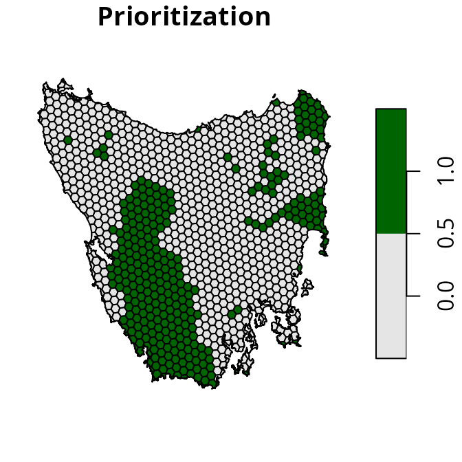
## # ℹ Use `summary(...)` to see complete formulation.

Prioritization

We can now solve the problem formulation (p1) to generate a prioritization (using the solve() function). The prioritizr R package supports a range of different exact algorithm solvers, including Gurobi, IBM CPLEX, CBC, HiGHS, Rsymphony, and lpsymphony. Although there are benefits and limitations associated with each of these different solvers, they should return similar results. Note that you will need at least one solver installed on your system to generate prioritizations. Since we did not specify a solver when building the problem, the prioritizr R package will automatically select the best available solver installed. We recommend using the Gurobi solver if possible, and have used it for this tutorial (see the Gurobi Installation Guide vignette for installation instructions). After solving the problem, the prioritization will be stored in the solution_1 column of the s1 object.

# solve problem
s1 <- solve(p1)

## Set parameter Username
## Set parameter LicenseID to value 2738655
## Set parameter TimeLimit to value 2147483647
## Set parameter MIPGap to value 0.1
## Set parameter Presolve to value 2
## Set parameter Threads to value 1
## Academic license - for non-commercial use only - expires 2026-11-14
## Gurobi Optimizer version 13.0.0 build v13.0.0rc1 (linux64 - "Ubuntu 24.04.2 LTS")
## 
## CPU model: 11th Gen Intel(R) Core(TM) i7-1185G7 @ 3.00GHz, instruction set [SSE2|AVX|AVX2|AVX512]
## Thread count: 4 physical cores, 8 logical processors, using up to 1 threads
## 
## Non-default parameters:
## TimeLimit  2147483647
## MIPGap  0.1
## Presolve  2
## Threads  1
## 
## Optimize a model with 6329 rows, 4278 columns and 20749 nonzeros (Min)
## Model fingerprint: 0xdea3ac39
## Model has 4278 linear objective coefficients
## Variable types: 3148 continuous, 1130 integer (1130 binary)
## Coefficient statistics:
##   Matrix range     [2e-06, 6e+01]
##   Objective range  [5e-01, 2e+02]
##   Bounds range     [1e+00, 1e+00]
##   RHS range        [2e-01, 2e+03]
## Found heuristic solution: objective 28313.965155
## Found heuristic solution: objective 18343.093396
## Presolve removed 1909 rows and 1249 columns
## Presolve time: 0.06s
## Presolved: 4420 rows, 3029 columns, 11081 nonzeros
## Found heuristic solution: objective 17798.824635
## Variable types: 0 continuous, 3029 integer (3029 binary)
## Found heuristic solution: objective 17508.673350
## Root relaxation presolve removed 8 rows and 6 columns
## Root relaxation presolved: 4412 rows, 3023 columns, 11060 nonzeros
## 
## 
## Root relaxation: objective 9.520699e+03, 1230 iterations, 0.05 seconds (0.08 work units)
## 
##     Nodes    |    Current Node    |     Objective Bounds      |     Work
##  Expl Unexpl |  Obj  Depth IntInf | Incumbent    BestBd   Gap | It/Node Time
## 
##      0     0 9520.69856    0 1115 17508.6734 9520.69856  45.6%     -    0s
## H    0     0                    13545.245401 9520.69856  29.7%     -    0s
## H    0     0                    12933.143362 9520.69856  26.4%     -    0s
## H    0     0                    12890.484624 9520.69856  26.1%     -    0s
## H    0     0                    12552.758530 9520.69856  24.2%     -    0s
##      0     0 9615.33215    0 1144 12552.7585 9615.33215  23.4%     -    0s
## H    0     0                    12507.566404 9615.33215  23.1%     -    0s
## H    0     0                    11563.819178 9615.33215  16.8%     -    0s
## H    0     0                    11369.016984 9615.33215  15.4%     -    0s
## H    0     0                    11366.954539 9615.33215  15.4%     -    0s
## H    0     0                    10939.351086 9615.33215  12.1%     -    0s
## H    0     0                    10907.751816 9615.33215  11.8%     -    0s
## H    0     0                    10861.560322 9615.33215  11.5%     -    0s
## H    0     0                    10858.199126 9615.33215  11.4%     -    0s
## H    0     0                    10810.254452 9615.33215  11.1%     -    0s
## H    0     0                    10806.686406 9615.33215  11.0%     -    0s
## H    0     0                    10699.834790 9615.33215  10.1%     -    0s
##      0     0 9617.05045    0 1157 10699.8348 9617.05045  10.1%     -    0s
##      0     0 9617.05168    0 1157 10699.8348 9617.05168  10.1%     -    0s
##      0     0 9624.88617    0 1057 10699.8348 9624.88617  10.0%     -    0s
## H    0     0                    10687.018567 9624.88617  9.94%     -    0s
## 
## Cutting planes:
##   Cover: 2
##   MIR: 1
##   RLT: 3
## 
## Explored 1 nodes (1498 simplex iterations) in 0.59 seconds (1.28 work units)
## Thread count was 1 (of 8 available processors)
## 
## Solution count 10: 10687 10699.8 10806.7 ... 11369
## 
## Optimal solution found (tolerance 1.00e-01)
## Best objective 1.068701856687e+04, best bound 9.624886170910e+03, gap 9.9385%

# plot map of prioritization
plot(
  st_as_sf(s1[, "solution_1"]), main = "Prioritization",
  pal = c("grey90", "darkgreen")
)

Feature representation

Let’s examine how well the vegetation communities are represented by existing protected areas and the prioritization.

# create column with existing protected areas
tas_pu$pa <- round(tas_pu$locked_in)

# calculate feature representation statistics based on existing protected areas
tc_pa <- eval_target_coverage_summary(p1, tas_pu[, "pa"])
print(tc_pa)

## # A tibble: 33 × 9
##    feature   met   total_amount absolute_target absolute_held absolute_shortfall
##    <chr>     <lgl>        <dbl>           <dbl>         <dbl>              <dbl>
##  1 Banksia … TRUE          2.00           0.340         0.367              0    
##  2 Boulders… TRUE        140.            23.9          65.5                0    
##  3 Callitri… FALSE         6.00           1.02          0.487              0.533
##  4 Cool tem… TRUE       7257.          1234.         2992.                 0    
##  5 Eucalypt… TRUE       5699.           969.         1398.                 0    
##  6 Eucalypt… FALSE      9180.          1561.         1030.               531.   
##  7 Eucalypt… TRUE         38.0            6.46         15.1                0    
##  8 Eucalypt… FALSE      1908.           324.          189.               135.   
##  9 Eucalypt… FALSE       388.            65.9          27.4               38.6  
## 10 Eucalypt… TRUE       6145.          1045.         1449.                 0    
## # ℹ 23 more rows
## # ℹ 3 more variables: relative_target <dbl>, relative_held <dbl>,
## #   relative_shortfall <dbl>

# calculate  feature representation statistics based on the prioritization
tc_s1 <- eval_target_coverage_summary(p1, s1[, "solution_1"])
print(tc_s1)

## # A tibble: 33 × 9
##    feature   met   total_amount absolute_target absolute_held absolute_shortfall
##    <chr>     <lgl>        <dbl>           <dbl>         <dbl>              <dbl>
##  1 Banksia … TRUE          2.00           0.340         0.367                  0
##  2 Boulders… TRUE        140.            23.9          70.8                    0
##  3 Callitri… TRUE          6.00           1.02          1.49                   0
##  4 Cool tem… TRUE       7257.          1234.         3255.                     0
##  5 Eucalypt… TRUE       5699.           969.         1772.                     0
##  6 Eucalypt… TRUE       9180.          1561.         1838.                     0
##  7 Eucalypt… TRUE         38.0            6.46         19.0                    0
##  8 Eucalypt… TRUE       1908.           324.          345.                     0
##  9 Eucalypt… TRUE        388.            65.9          79.5                    0
## 10 Eucalypt… TRUE       6145.          1045.         2083.                     0
## # ℹ 23 more rows
## # ℹ 3 more variables: relative_target <dbl>, relative_held <dbl>,
## #   relative_shortfall <dbl>

# explore representation by existing protected areas
## calculate number of features adequately represented by existing protected
## areas
sum(tc_pa$met)

## [1] 18

## summarize representation (values show percent coverage)
summary(tc_pa$relative_held * 100)

##    Min. 1st Qu.  Median    Mean 3rd Qu.    Max. 
##   0.000   3.163  18.363  23.827  39.649  93.002

## visualize representation  (values show percent coverage)
hist(tc_pa$relative_held * 100,
     main = "Feature representation by existing protected areas",
     xlim = c(0, 100),
     xlab = "Percent coverage of features (%)")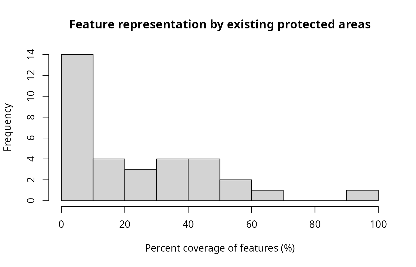

# explore representation by prioritization
## summarize representation (values show percent coverage)
summary(tc_s1$relative_held * 100)

##    Min. 1st Qu.  Median    Mean 3rd Qu.    Max. 
##   17.28   18.44   31.10   37.12   50.03  100.00

## calculate number of features adequately represented by the prioritization
sum(tc_s1$met)

## [1] 33

## visualize representation  (values show percent coverage)
hist(
  tc_s1$relative_held * 100,
  main = "Feature representation by prioritization",
  xlim = c(0, 100),
  xlab = "Percent coverage of features (%)"
)

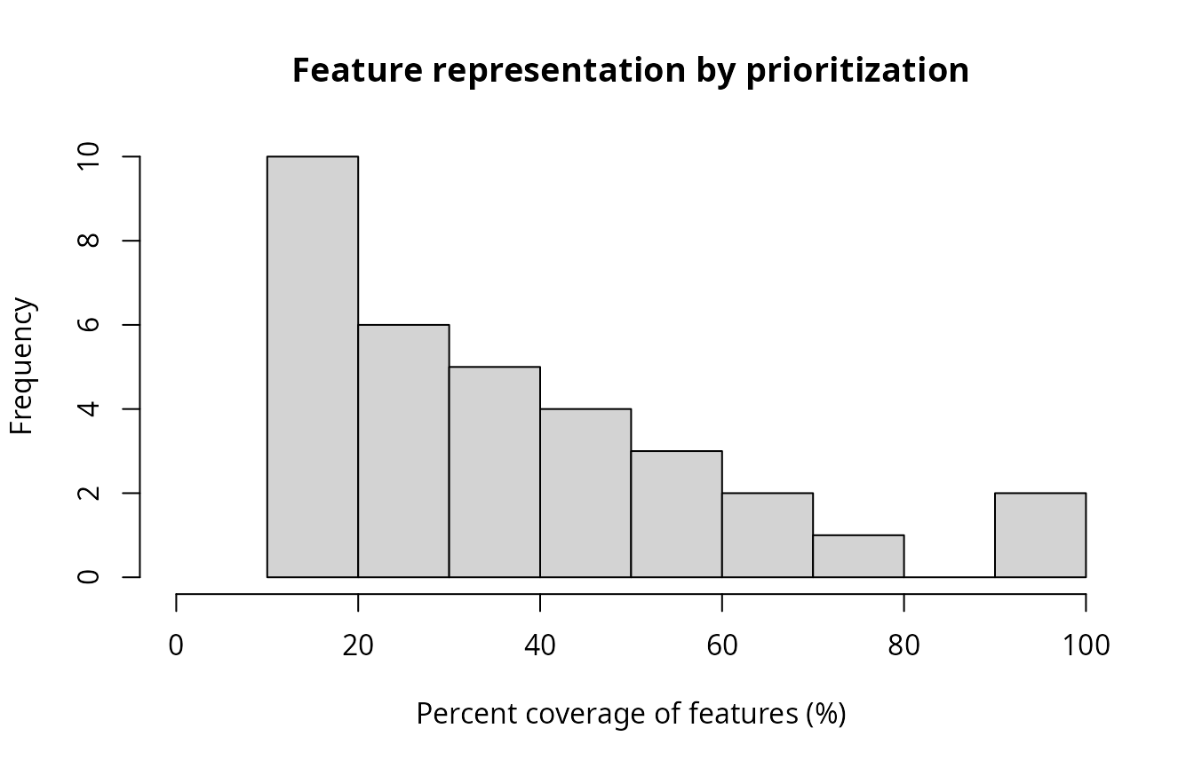
We can see that representation of the vegetation communities by existing protected areas is remarkably poor. For example, many of the vegetation communities have nearly zero coverage by existing protected areas. In other words, are almost entirely absent from existing protected areas. We can also see that all vegetation communities have at least 17% coverage by the prioritization – meaning that it meets the representation targets for all of the features.

Evaluating importance

After generating the prioritization, we can examine the relative importance of planning units selected by the prioritization. This can be useful to identify critically important planning units for conservation – in other words, places that contain biodiversity features which cannot be represented anywhere else – and schedule implementation of the prioritization. To achieve this, we will use an incremental rank approach (Jung et al. 2021). Briefly, this approach involves generating incremental prioritizations with increasing budgets, wherein planning units selected in a previous increment are locked in to the following solution. Additionally, locked out constraints are used to ensure that only planning units selected in the original solution are available for selection. If you’re interested, other approaches for examining importance are also available (see ?importance).

# calculate relative importance
imp_s1 <- eval_rank_importance(p1, s1["solution_1"], n = 10)
print(imp_s1)

# manually set locked in planning units to -1 to help with visualization,
# this way we can easily see the importance scores for the priority areas
imp_s1$rs[tas_pu$locked_in] <- -1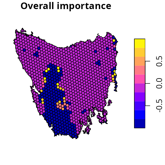

# plot map of importance scores
plot(st_as_sf(imp_s1[, "rs"]), main = "Overall importance")

Portfolios

Conservation planning exercises often involve generating multiple different prioritizations. This can help decision makers consider different options, and provide starting points for building consensus among stakeholders. To generate a range of different prioritizations given the same problem formulation, we can use portfolio functions. Here we will use the gap portfolio to generate 1000 solutions that are within 20% of optimality. Please note that you will need to have the Gurobi solver installed to use this specific portfolio. If you don’t have access to Gurobi, you could try using the shuffle portfolio instead (using the add_shuffle_portfolio() function).

# create new problem with a portfolio added to it
p2 <-
  p1 %>%
  add_gap_portfolio(number_solutions = 1000, pool_gap = 0.2)

# print problem
print(p2)

## A conservation problem (<ConservationProblem>)
## ├•data
## │├•features:    "Banksia woodlands", … (33 total)
## │└•planning units:
## │ ├•data:       <sf> (1130 total)
## │ ├•costs:      continuous values (between 0 and 61.92727)
## │ ├•extent:     298809.6, 5167775, 613818.8, 5502544 (xmin, ymin, xmax, ymax)
## │ └•CRS:        WGS 84 / UTM zone 55S (projected)
## ├•formulation
## │├•objective:   minimum set objective
## │├•penalties:
## ││└•1:          boundary penalties (`penalty` = 0.005, `edge_factor` = 0.5, `formulation` = "simple", …)
## │├•features:
## ││├•targets:    relative targets (all equal to 0.17)
## ││└•weights:    none specified
## │├•constraints:
## ││└•1:          locked in constraints (257 planning units)
## │└•decisions:   binary decision
## └•optimization
##  ├•portfolio:   gap portfolio (`number_solutions` = 1000, `pool_gap` = 0.2)
##  └•solver:      gurobi solver (`gap` = 0.1, `time_limit` = 2147483647, `first_feasible` = FALSE, …)
## # ℹ Use `summary(...)` to see complete formulation.

# generate prioritizations
prt <- solve(p2)

## Set parameter Username
## Set parameter LicenseID to value 2738655
## Set parameter TimeLimit to value 2147483647
## Set parameter MIPGap to value 0.1
## Set parameter Presolve to value 2
## Set parameter Threads to value 1
## Set parameter PoolSolutions to value 1000
## Set parameter PoolSearchMode to value 2
## Set parameter PoolGap to value 0.2
## Academic license - for non-commercial use only - expires 2026-11-14
## Gurobi Optimizer version 13.0.0 build v13.0.0rc1 (linux64 - "Ubuntu 24.04.2 LTS")
## 
## CPU model: 11th Gen Intel(R) Core(TM) i7-1185G7 @ 3.00GHz, instruction set [SSE2|AVX|AVX2|AVX512]
## Thread count: 4 physical cores, 8 logical processors, using up to 1 threads
## 
## Non-default parameters:
## TimeLimit  2147483647
## MIPGap  0.1
## Presolve  2
## Threads  1
## PoolSolutions  1000
## PoolSearchMode  2
## PoolGap  0.2
## 
## Optimize a model with 6329 rows, 4278 columns and 20749 nonzeros (Min)
## Model fingerprint: 0xdea3ac39
## Model has 4278 linear objective coefficients
## Variable types: 3148 continuous, 1130 integer (1130 binary)
## Coefficient statistics:
##   Matrix range     [2e-06, 6e+01]
##   Objective range  [5e-01, 2e+02]
##   Bounds range     [1e+00, 1e+00]
##   RHS range        [2e-01, 2e+03]
## Found heuristic solution: objective 28313.965155
## Found heuristic solution: objective 18343.093396
## Presolve removed 1434 rows and 258 columns
## Presolve time: 0.01s
## Presolved: 4895 rows, 4020 columns, 12058 nonzeros
## Variable types: 3148 continuous, 872 integer (872 binary)
## Root relaxation presolved: 4895 rows, 4020 columns, 12058 nonzeros
## 
## 
## Root relaxation: objective 9.516231e+03, 1430 iterations, 0.06 seconds (0.10 work units)
## 
##     Nodes    |    Current Node    |     Objective Bounds      |     Work
##  Expl Unexpl |  Obj  Depth IntInf | Incumbent    BestBd   Gap | It/Node Time
## 
##      0     0 9516.23114    0  311 18343.0934 9516.23114  48.1%     -    0s
## H    0     0                    13639.424721 9516.23114  30.2%     -    0s
## H    0     0                    12501.341845 9516.23114  23.9%     -    0s
## H    0     0                    12233.515013 9516.23114  22.2%     -    0s
##      0     0 9564.51582    0  330 12233.5150 9564.51582  21.8%     -    0s
## H    0     0                    11843.700741 9564.68826  19.2%     -    0s
## H    0     0                    11798.635920 9564.68826  18.9%     -    0s
##      0     0 9616.33444    0  323 11798.6359 9616.33444  18.5%     -    0s
##      0     0 9624.88617    0  289 11798.6359 9624.88617  18.4%     -    0s
##      0     0 9627.57060    0  314 11798.6359 9627.57060  18.4%     -    0s
##      0     0 9630.97840    0  289 11798.6359 9630.97840  18.4%     -    0s
##      0     0 9633.36306    0  287 11798.6359 9633.36306  18.4%     -    0s
## H    0     0                    11708.165533 9633.74322  17.7%     -    0s
##      0     0 9633.74322    0  287 11708.1655 9633.74322  17.7%     -    0s
## H    0     0                    11462.888107 9633.74322  16.0%     -    0s
## H    0     0                    11311.492903 9633.74322  14.8%     -    0s
## H    0     0                    11223.974201 9633.74322  14.2%     -    0s
## H    0     0                    11176.464423 9633.74322  13.8%     -    0s
## H    0     0                    11112.227846 9633.74322  13.3%     -    0s
## H    0     0                    11112.220632 9633.74322  13.3%     -    0s
## H    0     0                    11101.823799 9633.74322  13.2%     -    0s
## H    0     0                    11101.136772 9633.74322  13.2%     -    0s
##      0     2 9633.74322    0  287 11101.1368 9633.74322  13.2%     -    0s
## H    9     9                    11052.179320 9681.85648  12.4%  70.3    0s
## H   20    20                    11049.615924 9681.85648  12.4%   112    0s
## H   20    20                    11035.337817 9681.85648  12.3%   112    0s
## H   27    27                    10894.286480 9681.85648  11.1%   105    0s
## H   27    27                    10885.137873 9681.85648  11.1%   105    0s
## H   31    31                    10879.879840 9681.85648  11.0%   122    1s
## H   35    35                    10692.995163 9681.85648  9.46%   127    1s
## H   35    35                    10657.288141 9681.85648  9.15%   127    1s
## H   35    35                    10596.430044 9681.85648  8.63%   127    1s
## H   48    48                    10524.835882 9681.85648  8.01%   118    1s
## H   48    48                    10510.076877 9681.85648  7.88%   118    1s
## H   48    48                    10503.646971 9681.85648  7.82%   118    1s
## H   48    48                    10489.372919 9681.85648  7.70%   118    1s
## H   48    48                    10468.425222 9681.85648  7.51%   118    1s
## H  582   581                    10447.410643 9681.87545  7.33%  32.1    2s
##    606    18 9927.25228   20  278 10447.4106 9727.12134  6.89%  36.7    5s
## H  607    17                    10391.627829 9727.12134  6.39%  36.6    5s
## H  664    74                    10382.118919 9727.12134  6.31%  42.1    6s
## H  664    74                    10363.910766 9727.12134  6.14%  42.1    6s
## H  676    86                    10363.902562 9727.12134  6.14%  42.6    6s
## H  676    86                    10350.158606 9727.12134  6.02%  42.6    6s
## H 1138   512                    10258.932319 9731.87054  5.14%  32.7    8s
## H 1138   485                    10086.884243 9731.87054  3.52%  32.7    8s
## H 1141   487                    10077.735636 9731.87054  3.43%  32.8    8s
## H 1141   477                    10036.376759 9731.87054  3.03%  32.8    8s
## H 1160   494                    10031.956217 9731.87054  2.99%  33.1    8s
## H 1975  1250                    10000.713415 9772.14422  2.29%  26.1    9s
## H 1975  1250                    9992.0469328 9772.14422  2.20%  26.1    9s
## H 1975  1239                    9959.8770815 9772.14422  1.88%  26.1    9s
## H 1975  1239                    9954.0029029 9772.14422  1.83%  26.1    9s
## H 1975  1239                    9951.6451277 9772.14422  1.80%  26.1    9s
##   1986  1252 10456.8585   95    5 9951.64513 9772.14422  1.80%  26.1   10s
## H 2730  1750                    9948.6785488 9797.83470  1.52%  23.8   11s
## 
## Cutting planes:
##   Cover: 1
##   MIR: 3
##   RLT: 7
## 
## Explored 3606 nodes (92563 simplex iterations) in 13.40 seconds (18.18 work units)
## Thread count was 1 (of 8 available processors)
## 
## Solution count 1000: 9948.68 9951.65 9954 ... 10916.1
## No other solutions better than 10916.1
## 
## Optimal solution found (tolerance 1.00e-01)
## Best objective 9.948678548832e+03, best bound 9.825191496214e+03, gap 1.2412%

print(prt)

## Simple feature collection with 1130 features and 1004 fields
## Geometry type: MULTIPOLYGON
## Dimension:     XY
## Bounding box:  xmin: 298809.6 ymin: 5167775 xmax: 613818.8 ymax: 5502544
## Projected CRS: WGS 84 / UTM zone 55S
## # A tibble: 1,130 × 1,005
##       id  cost locked_in locked_out solution_1 solution_2 solution_3 solution_4
##  * <int> <dbl> <lgl>     <lgl>           <dbl>      <dbl>      <dbl>      <dbl>
##  1     1 60.2  FALSE     TRUE                0          0          0          0
##  2     2 19.9  FALSE     FALSE               0          0          0          0
##  3     3 59.7  FALSE     TRUE                0          0          0          0
##  4     4 32.4  FALSE     FALSE               0          0          0          0
##  5     5 26.2  FALSE     FALSE               0          0          0          0
##  6     6 51.3  FALSE     FALSE               0          0          0          0
##  7     7 32.3  FALSE     FALSE               0          0          0          0
##  8     8 38.4  FALSE     FALSE               0          0          0          0
##  9     9  3.55 FALSE     FALSE               0          0          0          0
## 10    10  1.83 FALSE     FALSE               0          0          0          0
## # ℹ 1,120 more rows
## # ℹ 997 more variables: solution_5 <dbl>, solution_6 <dbl>, solution_7 <dbl>,
## #   solution_8 <dbl>, solution_9 <dbl>, solution_10 <dbl>, solution_11 <dbl>,
## #   solution_12 <dbl>, solution_13 <dbl>, solution_14 <dbl>, solution_15 <dbl>,
## #   solution_16 <dbl>, solution_17 <dbl>, solution_18 <dbl>, solution_19 <dbl>,
## #   solution_20 <dbl>, solution_21 <dbl>, solution_22 <dbl>, solution_23 <dbl>,
## #   solution_24 <dbl>, solution_25 <dbl>, solution_26 <dbl>, …

After generating all these prioritizations, we now want some way to visualize them. Because it would be onerous to look at each and every prioritization individually, we will use statistical analyses to help us. We can visualize the differences between these different prioritizations – based on which planning units they selected – using a hierarchical cluster analysis (Harris et al. 2014).

# extract solutions
prt_results <- sf::st_drop_geometry(prt)
prt_results <- prt_results[, startsWith(names(prt_results), "solution_")]

# calculate pair-wise distances between different prioritizations for analysis
prt_dists <- vegan::vegdist(t(prt_results), method = "jaccard", binary = TRUE)

# run cluster analysis
prt_clust <- hclust(as.dist(prt_dists), method = "average")

# visualize clusters
opar <- par()
par(oma = c(0, 0, 0, 0), mar= c(0, 4.1, 1.5, 2.1))
plot(
  prt_clust, labels = FALSE, sub = NA, xlab = "",
  main = "Different prioritizations in portfolio"
)
suppressWarnings(par(opar))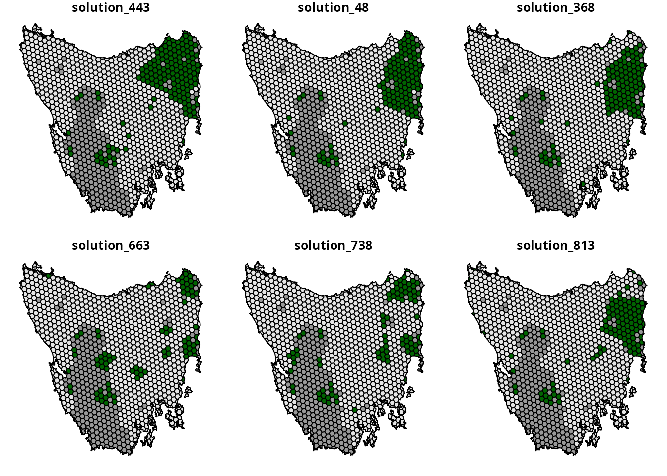

We can see that there are approximately six main groups of prioritizations in the portfolio. To explore these different groups, let’s conduct another cluster analysis (i.e., a k-medoids analysis) to extract the most representative prioritization from each of these groups. In other words, we will run another statistical analysis to find the most central prioritization within each group.

# run k-medoids analysis
prt_med <- pam(prt_dists, k = 6)

# extract names of prioritizations that are most central for each group.
prt_med_names <- prt_med$medoids
print(prt_med_names)

## [1] "solution_20"  "solution_127" "solution_521" "solution_57"  "solution_695"
## [6] "solution_219"

# create a copy of prt and set values for locked in planning units to -1
# so we can easily visualize differences between prioritizations
prt2 <- prt[, prt_med_names]
prt2[which(tas_pu$locked_in > 0.5), prt_med_names] <- -1

# plot a map showing main different prioritizations
# dark grey: locked in planning units
# grey: planning units not selected
# green: selected planning units
plot(st_as_sf(prt2), pal = c("grey60", "grey90", "darkgreen"))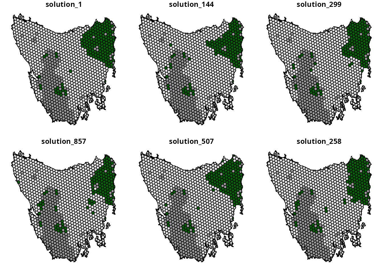

Marxan compatibility

The prioritizr R package provides functionality to help Marxan users generate prioritizations. Specifically, it can import conservation planning data prepared for Marxan, and can generate prioritizations using a similar problem formulation as Marxan (based on Beyer et al. 2016). Indeed, the problem formulation presented earlier in this vignette is very similar to that used by Marxan. The key difference is that the problem formulation we specified earlier uses “hard constraints” for feature representation, and Marxan uses “soft constraints” for feature representation. This means that prioritization we generated earlier was mathematically guaranteed to reach the targets for all features. However, if we used Marxan to generate the prioritization, then we could have produced a prioritization that would fail to reach targets (depending the Species Penalty Factors used to generate the prioritization). In addition to these differences in terms problem formulation, the prioritizr R package uses exact algorithms – instead of the simulated annealing algorithm – which ensures that we obtain prioritizations that are near optimal.

Here we will show the prioritizr R package can import Marxan data and generate a prioritization. To begin with, let’s import a conservation planning data prepared for Marxan.

# import data
## planning unit data
pu_path <- system.file("extdata/marxan/input/pu.dat", package = "prioritizr")
pu_data <- read.csv(pu_path, header = TRUE, stringsAsFactors = FALSE)
print(head(pu_data))

##   id       cost status    xloc     yloc
## 1  3      0.000      0 1116623 -4493479
## 2 30   7527.275      3 1110623 -4496943
## 3 56  37349.075      0 1092623 -4500408
## 4 58  16959.021      0 1116623 -4500408
## 5 84  34220.256      0 1098623 -4503872
## 6 85 178907.584      0 1110623 -4503872

## feature data
spec_path <- system.file(
  "extdata/marxan/input/spec.dat", package = "prioritizr"
)
spec_data <- read.csv(spec_path, header = TRUE, stringsAsFactors = FALSE)
print(head(spec_data))

##   id prop spf   name
## 1 10  0.3   1  bird1
## 2 11  0.3   1  nvis2
## 3 12  0.3   1  nvis8
## 4 13  0.3   1  nvis9
## 5 14  0.3   1 nvis14
## 6 15  0.3   1 nvis20

## amount of each feature within each planning unit data
puvspr_path <- system.file(
  "extdata/marxan/input/puvspr.dat", package = "prioritizr"
)
puvspr_data <- read.csv(puvspr_path, header = TRUE, stringsAsFactors = FALSE)
print(head(puvspr_data))

##   species  pu     amount
## 1      26  56 120.344884
## 2      26  58  45.167010
## 3      26  84  68.047375
## 4      26  85   9.735624
## 5      26  86   7.803476
## 6      26 111 478.327417

## boundary data
bound_path <- system.file(
  "extdata/marxan/input/bound.dat", package = "prioritizr"
)
bound_data <- read.table(bound_path, header = TRUE, stringsAsFactors = FALSE)
print(head(bound_data))

##   id1 id2 boundary
## 1   3   3    16000
## 2   3  30     4000
## 3   3  58     4000
## 4  30  30    12000
## 5  30  58     4000
## 6  30  85     4000

After importing the data, we can now generate a prioritization based on the Marxan problem formulation (using the marxan_problem() function). Please note that this function does not generate prioritizations using Marxan. Instead, it uses the data to create an optimization problem formulation similar to Marxan – using hard constraints instead of soft constraints – and uses an exact algorithm solver to generate a prioritization.

# create problem
p3 <- marxan_problem(
  pu_data, spec_data, puvspr_data, bound_data, blm = 0.0005
)

# print problem
print(p3)

## A conservation problem (<ConservationProblem>)
## ├•data
## │├•features:    "bird1", "nvis2", "nvis8", "nvis9", "nvis14", "nvis20", … (17 total)
## │└•planning units:
## │ ├•data:       <data.frame> (1751 total)
## │ ├•costs:      continuous values (between 0 and 415692.2)
## │ ├•extent:     NA
## │ └•CRS:        NA
## ├•formulation
## │├•objective:   minimum set objective
## │├•penalties:
## ││└•1:          boundary penalties (`penalty` = 0.0005, `edge_factor` = 1, `formulation` = "simple", …)
## │├•features:
## ││├•targets:    relative targets (all equal to 0.3)
## ││└•weights:    none specified
## │├•constraints:
## ││├•1:          locked in constraints (317 planning units)
## ││└•2:          locked out constraints (1 planning units)
## │└•decisions:   binary decision
## └•optimization
##  ├•portfolio:   default portfolio
##  └•solver:      gurobi solver (`gap` = 0.1, `time_limit` = 2147483647, `first_feasible` = FALSE, …)
## # ℹ Use `summary(...)` to see complete formulation.

# solve problem
s3 <- solve(p3)

## Set parameter Username
## Set parameter LicenseID to value 2738655
## Set parameter TimeLimit to value 2147483647
## Set parameter MIPGap to value 0.1
## Set parameter Presolve to value 2
## Set parameter Threads to value 1
## Academic license - for non-commercial use only - expires 2026-11-14
## Gurobi Optimizer version 13.0.0 build v13.0.0rc1 (linux64 - "Ubuntu 24.04.2 LTS")
## 
## CPU model: 11th Gen Intel(R) Core(TM) i7-1185G7 @ 3.00GHz, instruction set [SSE2|AVX|AVX2|AVX512]
## Thread count: 4 physical cores, 8 logical processors, using up to 1 threads
## 
## Non-default parameters:
## TimeLimit  2147483647
## MIPGap  0.1
## Presolve  2
## Threads  1
## 
## Optimize a model with 10075 rows, 6780 columns and 24778 nonzeros (Min)
## Model fingerprint: 0xe84a83d7
## Model has 6780 linear objective coefficients
## Variable types: 5029 continuous, 1751 integer (1751 binary)
## Coefficient statistics:
##   Matrix range     [5e-05, 4e+03]
##   Objective range  [4e+00, 4e+05]
##   Bounds range     [1e+00, 1e+00]
##   RHS range        [5e+03, 3e+05]
## Found heuristic solution: objective 1.221202e+08
## Presolve removed 4707 rows and 3103 columns
## Presolve time: 0.05s
## Presolved: 5368 rows, 3677 columns, 12704 nonzeros
## Variable types: 0 continuous, 3677 integer (3677 binary)
## Root relaxation presolved: 5368 rows, 3677 columns, 12704 nonzeros
## 
## 
## Root relaxation: objective 9.564790e+07, 521 iterations, 0.01 seconds (0.01 work units)
## 
##     Nodes    |    Current Node    |     Objective Bounds      |     Work
##  Expl Unexpl |  Obj  Depth IntInf | Incumbent    BestBd   Gap | It/Node Time
## 
##      0     0 9.5648e+07    0   20 1.2212e+08 9.5648e+07  21.7%     -    0s
## H    0     0                    9.660231e+07 9.5648e+07  0.99%     -    0s
## 
## Explored 1 nodes (521 simplex iterations) in 0.07 seconds (0.11 work units)
## Thread count was 1 (of 8 available processors)
## 
## Solution count 3: 9.66023e+07 9.66023e+07 1.2212e+08 
## 
## Optimal solution found (tolerance 1.00e-01)
## Best objective 9.660230173667e+07, best bound 9.564790440581e+07, gap 0.9880%

# print first six rows of solution object
print(head(s3))

## # A tibble: 6 × 8
##      id    cost status     xloc      yloc locked_in locked_out solution_1
##   <int>   <dbl>  <int>    <dbl>     <dbl> <lgl>     <lgl>           <dbl>
## 1     3      0       0 1116623. -4493479. FALSE     FALSE               0
## 2    30   7527.      3 1110623. -4496943. FALSE     TRUE                0
## 3    56  37349.      0 1092623. -4500408. FALSE     FALSE               1
## 4    58  16959.      0 1116623. -4500408. FALSE     FALSE               0
## 5    84  34220.      0 1098623. -4503872. FALSE     FALSE               0
## 6    85 178908.      0 1110623. -4503872. FALSE     FALSE               0

Conclusion

This tutorial shows how the prioritizr R package can be used to build a conservation problem, generate a prioritization, and evaluate it. Although we explored just a few functions, the package provides many different functions so that you can build and custom-tailor conservation planning problems to suit your needs. To learn more about the package, please see the package vignettes for an overview of the package, instructions for installing the Gurobi optimization suite, benchmarks comparing the performance of different solvers, and a record of publications that have cited the package. In addition to this tutorial, the package also provides tutorials on incorporating connectivity into prioritizations, calibrating trade-offs between different criteria (e.g., total cost and spatial fragmentation), and creating prioritizations that have multiple management zones or management actions.

References

Ball, I.R., Possingham, H. & Watts, M.E. (2009). Marxan and relatives: Software for spatial conservation prioritisation. Spatial Conservation Prioritisation: Quantitative Methods & Computational Tools (eds A. Moilanen, K.A. Wilson & H. Possingham), pp. 185–189. Oxford University Press, Oxford, UK.

Beyer, H.L., Dujardin, Y., Watts, M.E. & Possingham, H.P. (2016). Solving conservation planning problems with integer linear programming. Ecological Modelling, 328, 14–22.

Harris, L.R., Watts, M.E., Nel, R., Schoeman, D.S. & Possingham, H.P. (2014). Using multivariate statistics to explore trade-offs among spatial planning scenarios (P. Armsworth, Ed.). Journal of Applied Ecology, 51, 1504–1514.

Jung, M., Arnell, A., Lamo, X. de, García-Rangel, S., Lewis, M., Mark, J., Merow, C., Miles, L., Ondo, I., Pironon, S., Ravilious, C., Rivers, M., Schepaschenko, D., Tallowin, O., Soesbergen, A. van, Govaerts, R., Boyle, B.L., Enquist, B.J., Feng, X., Gallagher, R., Maitner, B., Meiri, S., Mulligan, M., Ofer, G., Roll, U., Hanson, J.O., Jetz, W., Di Marco, M., McGowan, J., Rinnan, D.S., Sachs, J.D., Lesiv, M., Adams, V.M., Andrew, S.C., Burger, J.R., Hannah, L., Marquet, P.A., McCarthy, J.K., Morueta-Holme, N., Newman, E.A., Park, D.S., Roehrdanz, P.R., Svenning, J.-C., Violle, C., Wieringa, J.J., Wynne, G., Fritz, S., Strassburg, B.B.N., Obersteiner, M., Kapos, V., Burgess, N., Schmidt-Traub, G. & Visconti, P. (2021). Areas of global importance for conserving terrestrial biodiversity, carbon and water. Nature Ecology & Evolution, 5, 1499–1509.