Add constraints to a conservation planning problem to ensure
that specific planning units are selected (or allocated
to a specific zone) in the solution. For example, it may be desirable to
lock in planning units that are inside existing protected areas so that the
solution fills in the gaps in the existing reserve network. If specific
planning units should be locked out of a solution, use
add_locked_out_constraints(). For problems with non-binary
planning unit allocations (e.g., proportions), the
add_manual_locked_constraints() function can be used to lock
planning unit allocations to a specific value.
Usage
add_locked_in_constraints(x, locked_in)

# S4 method for class 'ConservationProblem,numeric'
add_locked_in_constraints(x, locked_in)

# S4 method for class 'ConservationProblem,logical'
add_locked_in_constraints(x, locked_in)

# S4 method for class 'ConservationProblem,matrix'
add_locked_in_constraints(x, locked_in)

# S4 method for class 'ConservationProblem,character'
add_locked_in_constraints(x, locked_in)

# S4 method for class 'ConservationProblem,Spatial'
add_locked_in_constraints(x, locked_in)

# S4 method for class 'ConservationProblem,sf'
add_locked_in_constraints(x, locked_in)

# S4 method for class 'ConservationProblem,Raster'
add_locked_in_constraints(x, locked_in)

# S4 method for class 'ConservationProblem,SpatRaster'
add_locked_in_constraints(x, locked_in)
Arguments
- x
problem()object.- locked_in
Object that specifies which planning units should be locked in. See the Data format section for more information.
Value
An updated problem() object with the constraints added to it.
Data format
The following formats can be used to specify locked_in.
locked_inas anumericvectorHere
numericvalues are used to specify which planning units should be locked for the solution. Ifxhasdata.frameplanning units, then these values must refer to values in theidcolumn of the planning unit data. Alternatively, ifxhassf::st_sf()ormatrixplanning units, then these values must refer to the row numbers of the planning unit data. Additionally, ifxhasnumericvector planning units, then these values must refer to the element indices of the planning unit data. Finally, ifxhasterra::rast()planning units, then these values must refer to cell indices. Note that this format is only compatible ifxhas a single zone.locked_inas alogicalvectorHere
TRUE/FALSEvalues are used to specify each if planning unit should be locked for the solution. Note thatxshould have aTRUEorFALSEvalue for planning unit inx. Note that this format is only compatible ifxhas a single zone.locked_inas amatrixobjectHere
TRUE/FALSEvalues are used to specify each if each planning unit should be locked to a particular zone for the solution. Each row corresponds to a planning unit, each column corresponds to a zone, and each cell indicates if the planning unit should be locked to a given zone.locked_inas acharactervectorHere column name(s) for the planning unit data in
xare used to specify if planning units should be locked for the solution. This format is only compatible ifxhas planning units insf::st_sf()ordata.frameformat. These columns must havelogical(i.e.,TRUE/FALSE) values indicating if planning units should be locked for the solution. Ifxhas a single zone,locked_inmust contain a single column name. Otherwise, ifxhas multiple zones,locked_inmust contain a column name for each zone.locked_inas asf::sf()objectHere geometries of
locked_inare used to specify which planning units should be locked for the solution. Specifically, planning units inxthat spatially intersect withlocked_inwill be locked (perintersecting_units()). Note that this option is only compatible ifxhas a single zone.locked_inas aterra::rast()objectHere the cells in
locked_inare used to lock planning units for the solution. Specifically, planning units inxthat intersect with cells inlocked_inthat have non-zero and non-missing (NA) values will be locked. Ifxhas a single zone, thenlocked_inmust have a single layer. Otherwise, ifxhas multiple zones, thenlocked_inmust have a layer for each zone. Note that iflocked_inhas multiple layers, each cell must only contain a non-zero value in a single layer. Additionally, if the planning unit data inxis aterra::rast()object, we recommend standardizing missing (NA) values inlocked_inwith them to ensure that missing (NA) are consistent across both objects.
See also
Other functions for adding constraints:
add_contiguity_constraints(),
add_cost_constraints(),
add_feature_contiguity_constraints(),
add_linear_constraints(),
add_locked_out_constraints(),
add_mandatory_allocation_constraints(),
add_manual_bounded_constraints(),
add_manual_locked_constraints(),
add_neighbor_constraints()
Examples
# set seed for reproducibility
set.seed(500)
# load data
sim_pu_polygons <- get_sim_pu_polygons()
sim_features <- get_sim_features()
sim_locked_in_raster <- get_sim_locked_in_raster()
sim_zones_pu_raster <- get_sim_zones_pu_raster()
sim_zones_pu_polygons <- get_sim_zones_pu_polygons()
sim_zones_features <- get_sim_zones_features()
# create minimal problem
p1 <-
problem(sim_pu_polygons, sim_features, "cost") %>%
add_min_set_objective() %>%
add_relative_targets(0.2) %>%
add_binary_decisions() %>%
add_default_solver(verbose = FALSE)
# create problem with added locked in constraints using integers
p2 <- p1 %>% add_locked_in_constraints(which(sim_pu_polygons$locked_in))
# create problem with added locked in constraints using a column name
p3 <- p1 %>% add_locked_in_constraints("locked_in")
# create problem with added locked in constraints using raster data
p4 <- p1 %>% add_locked_in_constraints(sim_locked_in_raster)
# create problem with added locked in constraints using spatial polygon data
locked_in <- sim_pu_polygons[sim_pu_polygons$locked_in == 1, ]
p5 <- p1 %>% add_locked_in_constraints(locked_in)
# solve problems
s1 <- solve(p1)
s2 <- solve(p2)
s3 <- solve(p3)
s4 <- solve(p4)
s5 <- solve(p5)
# create single object with all solutions
s6 <- sf::st_sf(
tibble::tibble(
s1 = s1$solution_1,
s2 = s2$solution_1,
s3 = s3$solution_1,
s4 = s4$solution_1,
s5 = s5$solution_1
),
geometry = sf::st_geometry(s1)
)
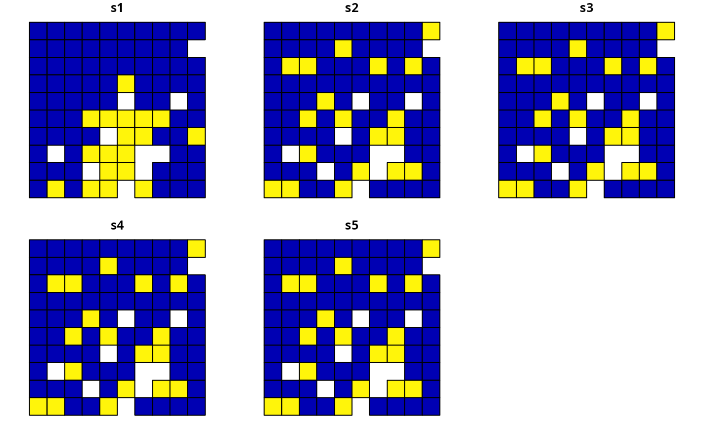
# plot solutions
plot(
s6,
main = c(
"none locked in", "locked in (integer input)",
"locked in (character input)", "locked in (raster input)",
"locked in (polygon input)"
)
)
 # create minimal multi-zone problem with spatial data
p7 <-
problem(
sim_zones_pu_polygons, sim_zones_features,
cost_column = c("cost_1", "cost_2", "cost_3")
) %>%
add_min_set_objective() %>%
add_absolute_targets(matrix(rpois(15, 1), nrow = 5, ncol = 3)) %>%
add_binary_decisions() %>%
add_default_solver(verbose = FALSE)
# create multi-zone problem with locked in constraints using matrix data
locked_matrix <- as.matrix(sf::st_drop_geometry(
sim_zones_pu_polygons[, c("locked_1", "locked_2", "locked_3")]
))
p8 <- p7 %>% add_locked_in_constraints(locked_matrix)
# solve problem
s8 <- solve(p8)
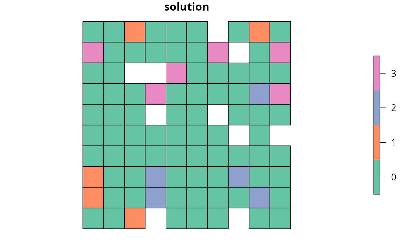
# create new column representing the zone id that each planning unit
# was allocated to in the solution
s8$solution <- category_vector(sf::st_drop_geometry(
s8[, c("solution_1_zone_1", "solution_1_zone_2", "solution_1_zone_3")]
))
s8$solution <- factor(s8$solution)
# plot solution
plot(s8[ "solution"], axes = FALSE)
# create minimal multi-zone problem with spatial data
p7 <-
problem(
sim_zones_pu_polygons, sim_zones_features,
cost_column = c("cost_1", "cost_2", "cost_3")
) %>%
add_min_set_objective() %>%
add_absolute_targets(matrix(rpois(15, 1), nrow = 5, ncol = 3)) %>%
add_binary_decisions() %>%
add_default_solver(verbose = FALSE)
# create multi-zone problem with locked in constraints using matrix data
locked_matrix <- as.matrix(sf::st_drop_geometry(
sim_zones_pu_polygons[, c("locked_1", "locked_2", "locked_3")]
))
p8 <- p7 %>% add_locked_in_constraints(locked_matrix)
# solve problem
s8 <- solve(p8)
# create new column representing the zone id that each planning unit
# was allocated to in the solution
s8$solution <- category_vector(sf::st_drop_geometry(
s8[, c("solution_1_zone_1", "solution_1_zone_2", "solution_1_zone_3")]
))
s8$solution <- factor(s8$solution)
# plot solution
plot(s8[ "solution"], axes = FALSE)
 # create multi-zone problem with locked in constraints using column names
p9 <- p7 %>% add_locked_in_constraints(c("locked_1", "locked_2", "locked_3"))
# solve problem
s9 <- solve(p9)
# create new column representing the zone id that each planning unit
# was allocated to in the solution
s9$solution <- category_vector(sf::st_drop_geometry(
s9[, c("solution_1_zone_1", "solution_1_zone_2", "solution_1_zone_3")]
))
s9$solution[s9$solution == 1 & s9$solution_1_zone_1 == 0] <- 0
s9$solution <- factor(s9$solution)
# plot solution
plot(s9[, "solution"], axes = FALSE)
# create multi-zone problem with raster planning units
p10 <-
problem(sim_zones_pu_raster, sim_zones_features) %>%
add_min_set_objective() %>%
add_absolute_targets(matrix(rpois(15, 1), nrow = 5, ncol = 3)) %>%
add_binary_decisions() %>%
add_default_solver(verbose = FALSE)
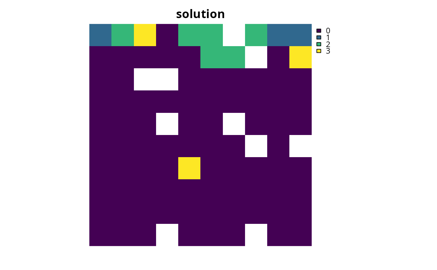
# create multi-layer raster with locked in units
locked_in_raster <- sim_zones_pu_raster[[1]]
locked_in_raster[!is.na(locked_in_raster)] <- 0
locked_in_raster <- locked_in_raster[[c(1, 1, 1)]]
names(locked_in_raster) <- c("zone_1", "zone_2", "zone_3")
locked_in_raster[[1]][1] <- 1
locked_in_raster[[2]][2] <- 1
locked_in_raster[[3]][3] <- 1
# plot locked in raster
plot(locked_in_raster)
# create multi-zone problem with locked in constraints using column names
p9 <- p7 %>% add_locked_in_constraints(c("locked_1", "locked_2", "locked_3"))
# solve problem
s9 <- solve(p9)
# create new column representing the zone id that each planning unit
# was allocated to in the solution
s9$solution <- category_vector(sf::st_drop_geometry(
s9[, c("solution_1_zone_1", "solution_1_zone_2", "solution_1_zone_3")]
))
s9$solution[s9$solution == 1 & s9$solution_1_zone_1 == 0] <- 0
s9$solution <- factor(s9$solution)
# plot solution
plot(s9[, "solution"], axes = FALSE)
# create multi-zone problem with raster planning units
p10 <-
problem(sim_zones_pu_raster, sim_zones_features) %>%
add_min_set_objective() %>%
add_absolute_targets(matrix(rpois(15, 1), nrow = 5, ncol = 3)) %>%
add_binary_decisions() %>%
add_default_solver(verbose = FALSE)
# create multi-layer raster with locked in units
locked_in_raster <- sim_zones_pu_raster[[1]]
locked_in_raster[!is.na(locked_in_raster)] <- 0
locked_in_raster <- locked_in_raster[[c(1, 1, 1)]]
names(locked_in_raster) <- c("zone_1", "zone_2", "zone_3")
locked_in_raster[[1]][1] <- 1
locked_in_raster[[2]][2] <- 1
locked_in_raster[[3]][3] <- 1
# plot locked in raster
plot(locked_in_raster)
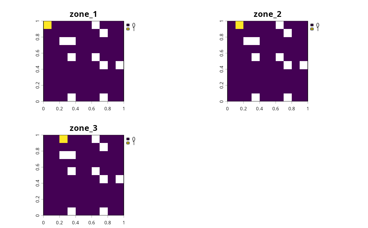 # add locked in raster units to problem
p10 <- p10 %>% add_locked_in_constraints(locked_in_raster)
# solve problem
s10 <- solve(p10)
# plot solution
plot(category_layer(s10), main = "solution", axes = FALSE)
# add locked in raster units to problem
p10 <- p10 %>% add_locked_in_constraints(locked_in_raster)
# solve problem
s10 <- solve(p10)
# plot solution
plot(category_layer(s10), main = "solution", axes = FALSE)