Add constraints to a conservation planning problem to ensure that all selected planning units meet certain criteria.
Usage
# S4 method for class 'ConservationProblem,ANY,ANY,character'
add_linear_constraints(x, threshold, sense, data)

# S4 method for class 'ConservationProblem,ANY,ANY,numeric'
add_linear_constraints(x, threshold, sense, data)

# S4 method for class 'ConservationProblem,ANY,ANY,matrix'
add_linear_constraints(x, threshold, sense, data)

# S4 method for class 'ConservationProblem,ANY,ANY,Matrix'
add_linear_constraints(x, threshold, sense, data)

# S4 method for class 'ConservationProblem,ANY,ANY,Raster'
add_linear_constraints(x, threshold, sense, data)

# S4 method for class 'ConservationProblem,ANY,ANY,SpatRaster'
add_linear_constraints(x, threshold, sense, data)

# S4 method for class 'ConservationProblem,ANY,ANY,dgCMatrix'
add_linear_constraints(x, threshold, sense, data)
Arguments
- x
problem()object.- threshold
numericvalue. This threshold value is also known as a "right-hand-side value" per integer programming terminology.- sense
charactervalue denoting the sense for the constraint. Acceptable values are:">=","<=", or"=".- data
charactervalue or vector,numericvector or matrix,terra::rast(), orMatrixobject containing the constraint values. These constraint values are also known as constraint coefficients per integer programming terminology. See the Data format section for more information.
Value
An updated problem() object with the constraints added to it.
Details
This function adds general purpose constraints that can be used to
ensure that solutions meet certain criteria
(see Examples section below for details).
For example, these constraints can be used to add multiple budgets.
They can also be used to ensure that the total number of planning units
allocated to a certain administrative area (e.g., country) does not exceed
a certain threshold (e.g., 30% of its total area). Furthermore,
they can also be used to ensure that features have a minimal level
of representation (e.g., 30%) when using an objective
function that aims to enhance feature representation given a budget
(e.g., add_min_shortfall_objective()).
Mathematical formulation
The linear constraints are implemented using the following
equation.
Let \(I\) denote the set of planning units
(indexed by \(i\)), \(Z\) the set of management zones (indexed by
\(z\)), and \(X_{iz}\) the decision variable for allocating
planning unit \(i\) to zone \(z\) (e.g., with binary
values indicating if each planning unit is allocated or not). Also, let
\(D_{iz}\) denote the constraint data associated with
planning units \(i \in I\) for zones \(z \in Z\)
(per data, if supplied as a matrix object),
\(\theta\) denote the constraint sense
(per sense), and \(t\) denote the constraint
threshold (per threshold).
$$ \sum_{i}^{I} \sum_{z}^{Z} (D_{iz} \times X_{iz}) \space \theta \space t $$
Data format
The following formats can be used to specify data.
dataas acharactervectorHere values are specified based on column name(s) for the planning unit data in
x. This format is only compatible if the planning units inxare asf::sf()ordata.frameobject. The column(s) must havenumericvalues, and must not contain any missing (NA) values. Ifxhas a single zone, thendatamust contain a single column name. Otherwise, ifxhas multiple zones, thendatamust contain a column name for each zone.dataas anumericvectorHere values are specified for each planning unit. These values must not contain any missing (
NA) values. Note that this format can only be used ifxhas a single zone.dataas amatrix/MatrixobjectHere values are specified for each planning unit and each zone. Note that
datamust havenumericvalues. Each row corresponds to a planning unit, each column corresponds to a zone, and each cell indicates the value associated with a planning unit when it is allocated to a given zone.dataas aterra::rast()objectHere values are specified for each planning unit and each zone. This format is only compatible if the planning units in
xaresf::sf(), orterra::rast()objects. If the planning unit data are asf::sf()object, then the values are calculated by overlaying the planning units withdataand calculating the sum of the values associated with each planning unit. If the planning unit data are aterra::rast()object, then the values are calculated by extracting the cell values (note thatdataand the planning unit inxmust have exactly the same dimensionality, extent, and missing values). Additionally, ifxhas multiple zones, thendatamust contain a layer for each zone.
See also
Other functions for adding constraints:
add_contiguity_constraints(),
add_cost_constraints(),
add_feature_contiguity_constraints(),
add_locked_in_constraints(),
add_locked_out_constraints(),
add_mandatory_allocation_constraints(),
add_manual_bounded_constraints(),
add_manual_locked_constraints(),
add_neighbor_constraints()
Examples
# load data
sim_pu_raster <- get_sim_pu_raster()
sim_features <- get_sim_features()
# create a baseline problem with minimum shortfall objective
p0 <-
problem(sim_pu_raster, sim_features) %>%
add_min_shortfall_objective(1800) %>%
add_relative_targets(0.2) %>%
add_binary_decisions() %>%
add_default_solver(verbose = FALSE)
# solve problem
s0 <- solve(p0)
# plot solution
plot(s0, main = "solution", axes = FALSE)
 # now let's create some modified versions of this baseline problem by
# adding additional criteria using linear constraints
# first, let's create a modified version of p0 that contains
# an additional budget for a secondary cost dataset
# create a secondary cost dataset by simulating values
sim_pu_raster2 <- simulate_cost(sim_pu_raster)
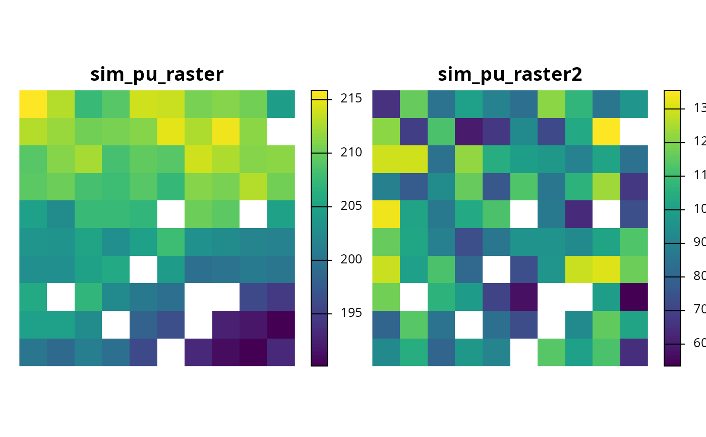
# plot the primary cost dataset (sim_pu_raster) and
# the secondary cost dataset (sim_pu_raster2)
plot(
c(sim_pu_raster, sim_pu_raster2),
main = c("sim_pu_raster", "sim_pu_raster2"),
axes = FALSE
)
# now let's create some modified versions of this baseline problem by
# adding additional criteria using linear constraints
# first, let's create a modified version of p0 that contains
# an additional budget for a secondary cost dataset
# create a secondary cost dataset by simulating values
sim_pu_raster2 <- simulate_cost(sim_pu_raster)
# plot the primary cost dataset (sim_pu_raster) and
# the secondary cost dataset (sim_pu_raster2)
plot(
c(sim_pu_raster, sim_pu_raster2),
main = c("sim_pu_raster", "sim_pu_raster2"),
axes = FALSE
)
 # create a modified version of p0 with linear constraints that
# specify that the planning units in the solution must not have
# values in sim_pu_raster2 that sum to a total greater than 500
p1 <-
p0 %>%
add_linear_constraints(
threshold = 500, sense = "<=", data = sim_pu_raster2
)
# solve problem
s1 <- solve(p1)
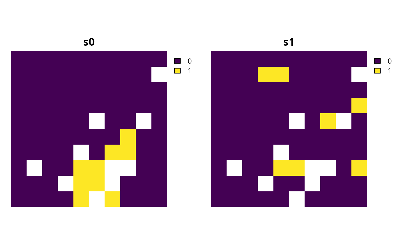
# plot solutions s1 and s2 to compare them
plot(c(s0, s1), main = c("s0", "s1"), axes = FALSE)
# create a modified version of p0 with linear constraints that
# specify that the planning units in the solution must not have
# values in sim_pu_raster2 that sum to a total greater than 500
p1 <-
p0 %>%
add_linear_constraints(
threshold = 500, sense = "<=", data = sim_pu_raster2
)
# solve problem
s1 <- solve(p1)
# plot solutions s1 and s2 to compare them
plot(c(s0, s1), main = c("s0", "s1"), axes = FALSE)
 # second, let's create a modified version of p0 that contains
# additional constraints to ensure that each feature definitely has
# at least 8% of its overall distribution represented by the solution
# (in addition to the 20% targets which specify how much we would
# ideally want to conserve for each feature)
# to achieve this, we need to calculate the total amount of each feature
# within the planning units so we can, in turn, set the constraint thresholds
feat_abund <- feature_abundances(p0)$absolute_abundance
# create a modified version of p0 with additional constraints for each
# feature to specify that the planning units in the solution must
# secure at least 8% of the total abundance for each feature
p2 <- p0
for (i in seq_len(terra::nlyr(sim_features))) {
p2 <-
p2 %>%
add_linear_constraints(
threshold = feat_abund[i] * 0.08,
sense = ">=",
data = sim_features[[i]]
)
}
# overall, p2 could be described as an optimization problem
# that maximizes feature representation as much as possible
# towards securing 20% of the total amount of each feature,
# whilst ensuring that (i) the total cost of the solution does
# not exceed 1800 (per cost values in sim_pu_raster) and (ii)
# the solution secures at least 8% of the total amount of each feature
# (if 20% is not possible due to the budget)
# solve problem
s2 <- solve(p2)
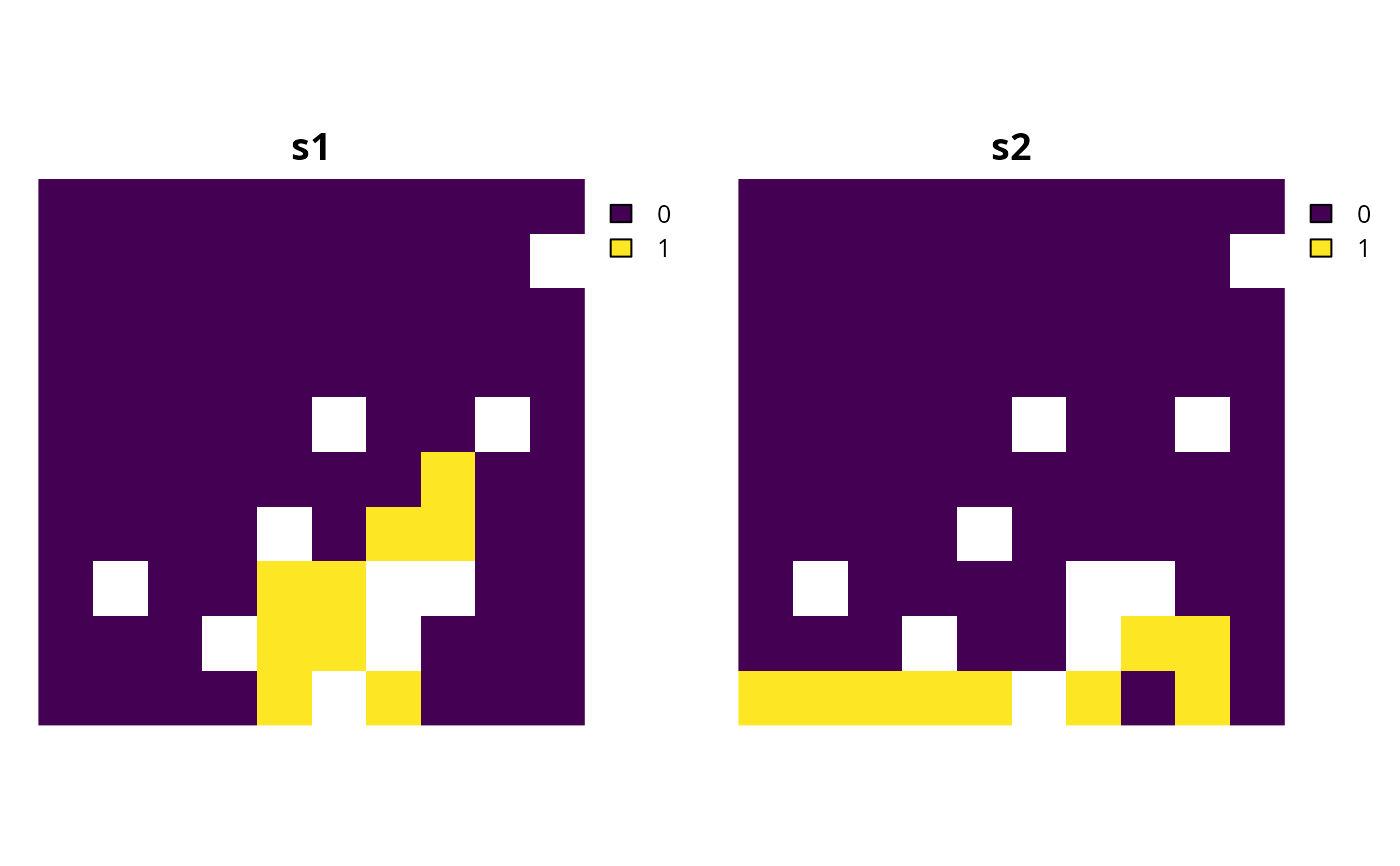
# plot solutions s0 and s2 to compare them
plot(c(s0, s2), main = c("s1", "s2"), axes = FALSE)
# second, let's create a modified version of p0 that contains
# additional constraints to ensure that each feature definitely has
# at least 8% of its overall distribution represented by the solution
# (in addition to the 20% targets which specify how much we would
# ideally want to conserve for each feature)
# to achieve this, we need to calculate the total amount of each feature
# within the planning units so we can, in turn, set the constraint thresholds
feat_abund <- feature_abundances(p0)$absolute_abundance
# create a modified version of p0 with additional constraints for each
# feature to specify that the planning units in the solution must
# secure at least 8% of the total abundance for each feature
p2 <- p0
for (i in seq_len(terra::nlyr(sim_features))) {
p2 <-
p2 %>%
add_linear_constraints(
threshold = feat_abund[i] * 0.08,
sense = ">=",
data = sim_features[[i]]
)
}
# overall, p2 could be described as an optimization problem
# that maximizes feature representation as much as possible
# towards securing 20% of the total amount of each feature,
# whilst ensuring that (i) the total cost of the solution does
# not exceed 1800 (per cost values in sim_pu_raster) and (ii)
# the solution secures at least 8% of the total amount of each feature
# (if 20% is not possible due to the budget)
# solve problem
s2 <- solve(p2)
# plot solutions s0 and s2 to compare them
plot(c(s0, s2), main = c("s1", "s2"), axes = FALSE)
 # third, let's create a modified version of p0 that contains
# additional constraints to ensure that the solution equitably
# distributes conservation effort across different administrative areas
# (e.g., countries) within the study region
# to begin with, we will simulate a dataset describing the spatial extent of
# four different administrative areas across the study region
sim_admin <- sim_pu_raster
sim_admin <- terra::aggregate(sim_admin, fact = 5)
sim_admin <- terra::setValues(sim_admin, seq_len(terra::ncell(sim_admin)))
sim_admin <- terra::resample(sim_admin, sim_pu_raster, method = "near")
sim_admin <- terra::mask(sim_admin, sim_pu_raster)
# plot administrative areas layer,
# we can see that the administrative areas subdivide
# the study region into four quadrants, and the sim_admin object is a
# SpatRaster with integer values denoting ids for the administrative areas
plot(sim_admin, axes = FALSE)
# third, let's create a modified version of p0 that contains
# additional constraints to ensure that the solution equitably
# distributes conservation effort across different administrative areas
# (e.g., countries) within the study region
# to begin with, we will simulate a dataset describing the spatial extent of
# four different administrative areas across the study region
sim_admin <- sim_pu_raster
sim_admin <- terra::aggregate(sim_admin, fact = 5)
sim_admin <- terra::setValues(sim_admin, seq_len(terra::ncell(sim_admin)))
sim_admin <- terra::resample(sim_admin, sim_pu_raster, method = "near")
sim_admin <- terra::mask(sim_admin, sim_pu_raster)
# plot administrative areas layer,
# we can see that the administrative areas subdivide
# the study region into four quadrants, and the sim_admin object is a
# SpatRaster with integer values denoting ids for the administrative areas
plot(sim_admin, axes = FALSE)
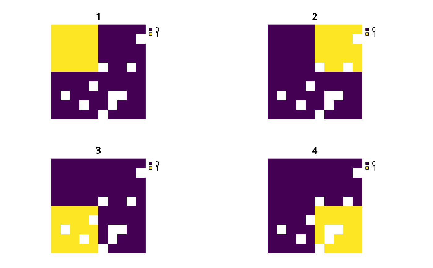
 # next we will convert the sim_admin SpatRaster object into a SpatRaster
# object (with a layer for each administrative area) indicating which
# planning units belong to each administrative area using binary
# (presence/absence) values
sim_admin2 <- binary_stack(sim_admin)
# plot binary stack of administrative areas
plot(sim_admin2, axes = FALSE)
# next we will convert the sim_admin SpatRaster object into a SpatRaster
# object (with a layer for each administrative area) indicating which
# planning units belong to each administrative area using binary
# (presence/absence) values
sim_admin2 <- binary_stack(sim_admin)
# plot binary stack of administrative areas
plot(sim_admin2, axes = FALSE)
 # we will now calculate the total amount of planning units associated
# with each administrative area, so that we can set the constraint threshold
# since we are using raster data, we won't bother explicitly
# accounting for the total area of each planning unit (because all
# planning units have the same area in raster formats) -- but if we were
# using vector data then we would need to account for the area of each unit
admin_total <- Matrix::rowSums(rij_matrix(sim_pu_raster, sim_admin2))
# create a modified version of p0 with additional constraints for each
# administrative area to specify that the planning units in the solution must
# not encompass more than 10% of the total extent of the administrative
# area
p3 <- p0
for (i in seq_len(terra::nlyr(sim_admin2))) {
p3 <-
p3 %>%
add_linear_constraints(
threshold = admin_total[i] * 0.1,
sense = "<=",
data = sim_admin2[[i]]
)
}
# solve problem
s3 <- solve(p3)
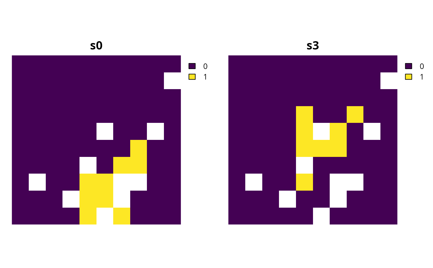
# plot solutions s0 and s3 to compare them
plot(c(s0, s3), main = c("s0", "s3"), axes = FALSE)
# we will now calculate the total amount of planning units associated
# with each administrative area, so that we can set the constraint threshold
# since we are using raster data, we won't bother explicitly
# accounting for the total area of each planning unit (because all
# planning units have the same area in raster formats) -- but if we were
# using vector data then we would need to account for the area of each unit
admin_total <- Matrix::rowSums(rij_matrix(sim_pu_raster, sim_admin2))
# create a modified version of p0 with additional constraints for each
# administrative area to specify that the planning units in the solution must
# not encompass more than 10% of the total extent of the administrative
# area
p3 <- p0
for (i in seq_len(terra::nlyr(sim_admin2))) {
p3 <-
p3 %>%
add_linear_constraints(
threshold = admin_total[i] * 0.1,
sense = "<=",
data = sim_admin2[[i]]
)
}
# solve problem
s3 <- solve(p3)
# plot solutions s0 and s3 to compare them
plot(c(s0, s3), main = c("s0", "s3"), axes = FALSE)