Add constraints to a conservation planning problem to ensure that all selected planning units in the solution each have, at least, a predefined number of neighbors that are also selected in the solution.
Usage
# S4 method for class 'ConservationProblem,ANY,ANY,ANY,ANY'
add_neighbor_constraints(x, k, clamp, zones, data)

# S4 method for class 'ConservationProblem,ANY,ANY,ANY,data.frame'
add_neighbor_constraints(x, k, clamp, zones, data)

# S4 method for class 'ConservationProblem,ANY,ANY,ANY,matrix'
add_neighbor_constraints(x, k, clamp, zones, data)

# S4 method for class 'ConservationProblem,ANY,ANY,ANY,array'
add_neighbor_constraints(x, k, clamp, zones, data)
Arguments
- x
problem()object.- k
integervalue denoting the minimum number of neighbors for selected planning units in the solution. Ifxhas multiple zones, thenkmust have a value for each zone.- clamp
logicalvalue indicating if the minimum number of neighbors for selected planning units be clamped to feasibility? For example, if a planning unit has only two neighbors,k = 3, andclamp = FALSE, then the planning unit could not ever be selected in the solution. However, ifclamp = TRUE, then the planning unit could potentially be selected in the solution if both of its two neighbors were also selected. Defaults toTRUE.- zones
matrixorMatrixobject describing the neighborhood scheme for different zones. Each row and column corresponds to a different zone inx, and cell values must contain binarynumericvalues (i.e., one or zero) that indicate if neighboring planning units (perdata) should be treated as neighbors if they are allocated to different zones. The cell values along the diagonal of the matrix indicate if planning units that are allocated to the same zone should be considered neighbors or not. Defaults to an identity matrix (i.e., a matrix with ones along the matrix diagonal and zeros elsewhere), so that planning units are only considered neighbors if they are both allocated to the same zone.- data
NULL,matrix,Matrix,data.frame, orarrayobject showing which planning units are neighbors with each other. Defaults toNULLsuch that the neighborhood data are calculated automatically using theadjacency_matrix()function. See the Data format section for more information.
Value
An updated problem() object with the constraints added to it.
Details
This function uses neighborhood data to identify solutions that surround planning units with a minimum number of neighbors. It was inspired by the mathematical formulations detailed in Billionnet (2013) and Beyer et al. (2016).
Data format
The following formats can be used to specify data.
dataas aNULLvalueHere the neighborhood data are calculated automatically using the
adjacency_matrix()function. This is the default fordata. Note that the neighborhood data must be manually defined using one of the other formats below if the planning unit data inxis not spatially referenced (e.g.,data.frameornumericformat).dataas amatrix/MatrixobjectHere rows and columns correspond to different planning units and cell values indicate if two planning units are neighbors or not. Cells must have binary
numericvalues (i.e., one or zero). Note that cells along the matrix diagonal have no effect on the solution because each planning unit cannot be a neighbor with itself.dataas adata.frameobjectHere rows correspond to a pair of planning units and columns provide information about each pair of planning units. In particular,
datamust have the columns:"id1","id2", and"boundary". The"id1"and"id2"columns contain identifiers (indices) for a pair of planning units, and the"boundary"column contains binarynumericvalues that indicate if the two planning units specified in the"id1"and"id2"columns should be treated as neighbors or not. These data can be used to describe symmetric or asymmetric relationships between planning units. By default, input data is assumed to be symmetric unless asymmetric data is specified (e.g., if data is present for planning units 2 and 3, then the same amount of connectivity is expected for planning units 3 and 2, unless connectivity data is also provided for planning units 3 and 2). Ifxhas multiple zones, then the "zone1"and"zone2"columns can optionally be provided to manually specify that the neighborhood data pertain to specific zones. The"zone1"and"zone2"columns should contain thecharacternames of the zones. Note that if the columns"zone1"and"zone2"are present, thenzonesmust beNULL`.dataas anarrayobjectHere a four-dimension array containing binary
numericvalues is used to specify if planning unit should be treated as neighbors with every other planning unit when they are allocated to every combination of management zone. The first two dimensions (i.e., rows and columns) correspond to the planning units, and second two dimensions correspond to the management zones. For example, ifdatahad a value of 1 at the indexdata[1, 2, 3, 4], this would indicate that planning unit 1 and planning unit 2 should be treated as neighbors when they are allocated to zones 3 and 4 (respectively).
References
Beyer HL, Dujardin Y, Watts ME, and Possingham HP (2016) Solving conservation planning problems with integer linear programming. Ecological Modelling, 228: 14–22.
Billionnet A (2013) Mathematical optimization ideas for biodiversity conservation. European Journal of Operational Research, 231: 514–534.
See also
Other functions for adding constraints:
add_contiguity_constraints(),
add_cost_constraints(),
add_feature_contiguity_constraints(),
add_linear_constraints(),
add_locked_in_constraints(),
add_locked_out_constraints(),
add_mandatory_allocation_constraints(),
add_manual_bounded_constraints(),
add_manual_locked_constraints()
Examples
# load data
sim_pu_raster <- get_sim_pu_raster()
sim_features <- get_sim_features()
sim_zones_pu_raster <- get_sim_zones_pu_raster()
sim_zones_features <- get_sim_zones_features()
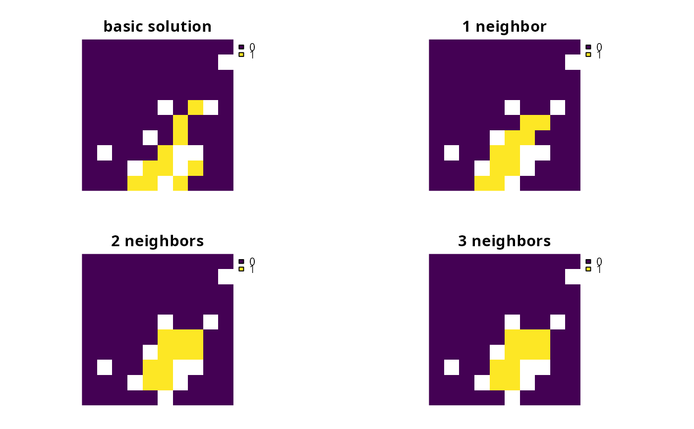
# create minimal problem
p1 <-
problem(sim_pu_raster, sim_features) %>%
add_min_set_objective() %>%
add_relative_targets(0.1) %>%
add_default_solver(verbose = FALSE)
# create problem with constraints that require 1 neighbor
# and neighbors are defined using a rook-style neighborhood
p2 <- p1 %>% add_neighbor_constraints(1)
# create problem with constraints that require 2 neighbor
# and neighbors are defined using a rook-style neighborhood
p3 <- p1 %>% add_neighbor_constraints(2)
# create problem with constraints that require 3 neighbor
# and neighbors are defined using a queen-style neighborhood
p4 <-
p1 %>%
add_neighbor_constraints(
3, data = adjacency_matrix(sim_pu_raster, directions = 8)
)
# solve problems
s1 <- c(solve(p1), solve(p2), solve(p3), solve(p4))
names(s1) <- c("basic solution", "1 neighbor", "2 neighbors", "3 neighbors")
# plot solutions
plot(s1, axes = FALSE)
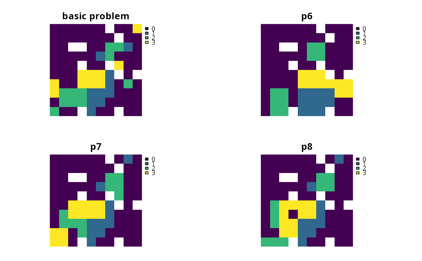
 # create minimal problem with multiple zones
p5 <-
problem(sim_zones_pu_raster, sim_zones_features) %>%
add_min_set_objective() %>%
add_relative_targets(matrix(0.1, ncol = 3, nrow = 5)) %>%
add_default_solver(verbose = FALSE)
# create problem where selected planning units require at least 2 neighbors
# for each zone and planning units are only considered neighbors if they
# are allocated to the same zone
z6 <- diag(3)
print(z6)
#> [,1] [,2] [,3]
#> [1,] 1 0 0
#> [2,] 0 1 0
#> [3,] 0 0 1
p6 <- p5 %>% add_neighbor_constraints(rep(2, 3), zones = z6)
# create problem where the planning units in zone 1 don't explicitly require
# any neighbors, planning units in zone 2 require at least 1 neighbors, and
# planning units in zone 3 require at least 2 neighbors. As before, planning
# units are still only considered neighbors if they are allocated to the
# same zone
p7 <- p5 %>% add_neighbor_constraints(c(0, 1, 2), zones = z6)
# create problem given the same constraints as outlined above, except
# that when determining which selected planning units are neighbors,
# planning units that are allocated to zone 1 and zone 2 can also treated
# as being neighbors with each other
z8 <- diag(3)
z8[1, 2] <- 1
z8[2, 1] <- 1
print(z8)
#> [,1] [,2] [,3]
#> [1,] 1 1 0
#> [2,] 1 1 0
#> [3,] 0 0 1
p8 <- p5 %>% add_neighbor_constraints(c(0, 1, 2), zones = z8)
# solve problems
s2 <- list(p5, p6, p7, p8)
s2 <- lapply(s2, solve)
s2 <- lapply(s2, category_layer)
s2 <- terra::rast(s2)
names(s2) <- c("basic problem", "p6", "p7", "p8")
# plot solutions
plot(s2, main = names(s2), axes = FALSE)
# create minimal problem with multiple zones
p5 <-
problem(sim_zones_pu_raster, sim_zones_features) %>%
add_min_set_objective() %>%
add_relative_targets(matrix(0.1, ncol = 3, nrow = 5)) %>%
add_default_solver(verbose = FALSE)
# create problem where selected planning units require at least 2 neighbors
# for each zone and planning units are only considered neighbors if they
# are allocated to the same zone
z6 <- diag(3)
print(z6)
#> [,1] [,2] [,3]
#> [1,] 1 0 0
#> [2,] 0 1 0
#> [3,] 0 0 1
p6 <- p5 %>% add_neighbor_constraints(rep(2, 3), zones = z6)
# create problem where the planning units in zone 1 don't explicitly require
# any neighbors, planning units in zone 2 require at least 1 neighbors, and
# planning units in zone 3 require at least 2 neighbors. As before, planning
# units are still only considered neighbors if they are allocated to the
# same zone
p7 <- p5 %>% add_neighbor_constraints(c(0, 1, 2), zones = z6)
# create problem given the same constraints as outlined above, except
# that when determining which selected planning units are neighbors,
# planning units that are allocated to zone 1 and zone 2 can also treated
# as being neighbors with each other
z8 <- diag(3)
z8[1, 2] <- 1
z8[2, 1] <- 1
print(z8)
#> [,1] [,2] [,3]
#> [1,] 1 1 0
#> [2,] 1 1 0
#> [3,] 0 0 1
p8 <- p5 %>% add_neighbor_constraints(c(0, 1, 2), zones = z8)
# solve problems
s2 <- list(p5, p6, p7, p8)
s2 <- lapply(s2, solve)
s2 <- lapply(s2, category_layer)
s2 <- terra::rast(s2)
names(s2) <- c("basic problem", "p6", "p7", "p8")
# plot solutions
plot(s2, main = names(s2), axes = FALSE)