Add feature contiguity constraints

Add constraints to a problem to ensure that each feature is represented in a contiguous unit of dispersible habitat. These constraints are a more advanced version of those implemented in the add_contiguity_constraints() function, because they ensure that each feature is represented in a contiguous unit and not that the entire solution should form a contiguous unit. Additionally, this function can use data showing the distribution of dispersible habitat for each feature to ensure that all features can disperse throughout the areas designated for their conservation.

Usage

# S4 method for ConservationProblem,ANY,data.frame
add_feature_contiguity_constraints(x, zones, data)

# S4 method for ConservationProblem,ANY,matrix
add_feature_contiguity_constraints(x, zones, data)

# S4 method for ConservationProblem,ANY,ANY
add_feature_contiguity_constraints(x, zones, data)

Arguments

x: problem() object.
zones: matrix, Matrix or list object describing the connection scheme for different zones. For matrix or and Matrix arguments, each row and column corresponds to a different zone in the argument to x, and cell values must contain binary numeric values (i.e., one or zero) that indicate if connected planning units (as specified in the argument to data) should be still considered connected if they are allocated to different zones. The cell values along the diagonal of the matrix indicate if planning units should be subject to contiguity constraints when they are allocated to a given zone. Note arguments to zones must be symmetric, and that a row or column has a value of one then the diagonal element for that row or column must also have a value of one. If the connection scheme between different zones should differ among the features, then the argument to zones should be a list of matrix or Matrix objects that shows the specific scheme for each feature using the conventions described above. The default argument to zones is an identity matrix (i.e., a matrix with ones along the matrix diagonal and zeros elsewhere), so that planning units are only considered connected if they are both allocated to the same zone.
data: NULL, matrix, Matrix, data.frame or list of matrix, Matrix, or data.frame objects. The argument to data shows which planning units should be treated as being connected when implementing constraints to ensure that features are represented in contiguous units. If different features have different dispersal capabilities, then it may be desirable to specify which sets of planning units should be treated as being connected for which features using a list of objects. The default argument is NULL which means that the connection data is calculated automatically using the adjacency_matrix() function and so all adjacent planning units are treated as being connected for all features. See the Data format section for more information.

Value

An updated problem() object with the constraints added to it.

Details

This function uses connection data to identify solutions that represent features in contiguous units of dispersible habitat. It was inspired by the mathematical formulations detailed in Önal and Briers (2006) and Cardeira et al. 2010. For an example that has used these constraints, see Hanson et al. (2019). Please note that these constraints require the expanded formulation and therefore cannot be used with feature data that have negative vales. Please note that adding these constraints to a problem will drastically increase the amount of time required to solve it.

Data format

The argument to data can be specified using the following formats.

data as a NULL value: connection data should be calculated automatically using the adjacency_matrix() function. This is the default argument and means that all adjacent planning units are treated as potentially dispersible for all features. Note that the connection data must be manually defined using one of the other formats below when the planning unit data in the argument to x is not spatially referenced (e.g., in data.frame or numeric format).
data as amatrix/Matrix object: where rows and columns represent different planning units and the value of each cell indicates if the two planning units are connected or not. Cell values should be binary numeric values (i.e., one or zero). Cells that occur along the matrix diagonal have no effect on the solution at all because each planning unit cannot be a connected with itself. Note that pairs of connected planning units are treated as being potentially dispersible for all features.
data as a data.frame object: containing columns that are named "id1", "id2", and "boundary". Here, each row denotes the connectivity between two planning units following the Marxan format. The "boundary" column should contain binary numeric values that indicate if the two planning units specified in the "id1" and "id2" columns are connected or not. This data can be used to describe symmetric or asymmetric relationships between planning units. By default, input data is assumed to be symmetric unless asymmetric data is also included (e.g., if data is present for planning units 2 and 3, then the same amount of connectivity is expected for planning units 3 and 2, unless connectivity data is also provided for planning units 3 and 2). Note that pairs of connected planning units are treated as being potentially dispersible for all features.
data as a list object: containing matrix, Matrix, or data.frame objects showing which planning units should be treated as connected for each feature. Each element in the list should correspond to a different feature (specifically, a different target in the problem), and should contain a matrix, Matrix, or data.frame object that follows the conventions detailed above.

Notes

In early versions, it was named as the add_corridor_constraints function.

References

Önal H and Briers RA (2006) Optimal selection of a connected reserve network. Operations Research, 54: 379--388.

Cardeira JO, Pinto LS, Cabeza M and Gaston KJ (2010) Species specific connectivity in reserve-network design using graphs. Biological Conservation, 2: 408--415.

Hanson JO, Fuller RA, & Rhodes JR (2019) Conventional methods for enhancing connectivity in conservation planning do not always maintain gene flow. Journal of Applied Ecology, 56: 913--922.

Examples

# \dontrun{
# load data
sim_pu_raster <- get_sim_pu_raster()
sim_features <- get_sim_features()
sim_zones_pu_raster <- get_sim_zones_pu_raster()
sim_zones_features <- get_sim_zones_features()

# create minimal problem
p1 <-
  problem(sim_pu_raster, sim_features) %>%
  add_min_set_objective() %>%
  add_relative_targets(0.3) %>%
  add_binary_decisions() %>%
  add_default_solver(verbose = FALSE)

# create problem with contiguity constraints
p2 <- p1 %>% add_contiguity_constraints()

# create problem with constraints to represent features in contiguous
# units
p3 <- p1 %>% add_feature_contiguity_constraints()

# create problem with constraints to represent features in contiguous
# units that contain highly suitable habitat values
# (specifically in the top 5th percentile)
cm4 <- lapply(seq_len(terra::nlyr(sim_features)), function(i) {
  # create connectivity matrix using the i'th feature's habitat data
  m <- connectivity_matrix(sim_pu_raster, sim_features[[i]])
  # convert matrix to 0/1 values denoting values in top 5th percentile
  m <- round(m > quantile(as.vector(m), 1 - 0.05, names = FALSE))
  # remove 0s from the sparse matrix
  m <- Matrix::drop0(m)
  # return matrix
  m
})
p4 <- p1 %>% add_feature_contiguity_constraints(data = cm4)

# solve problems
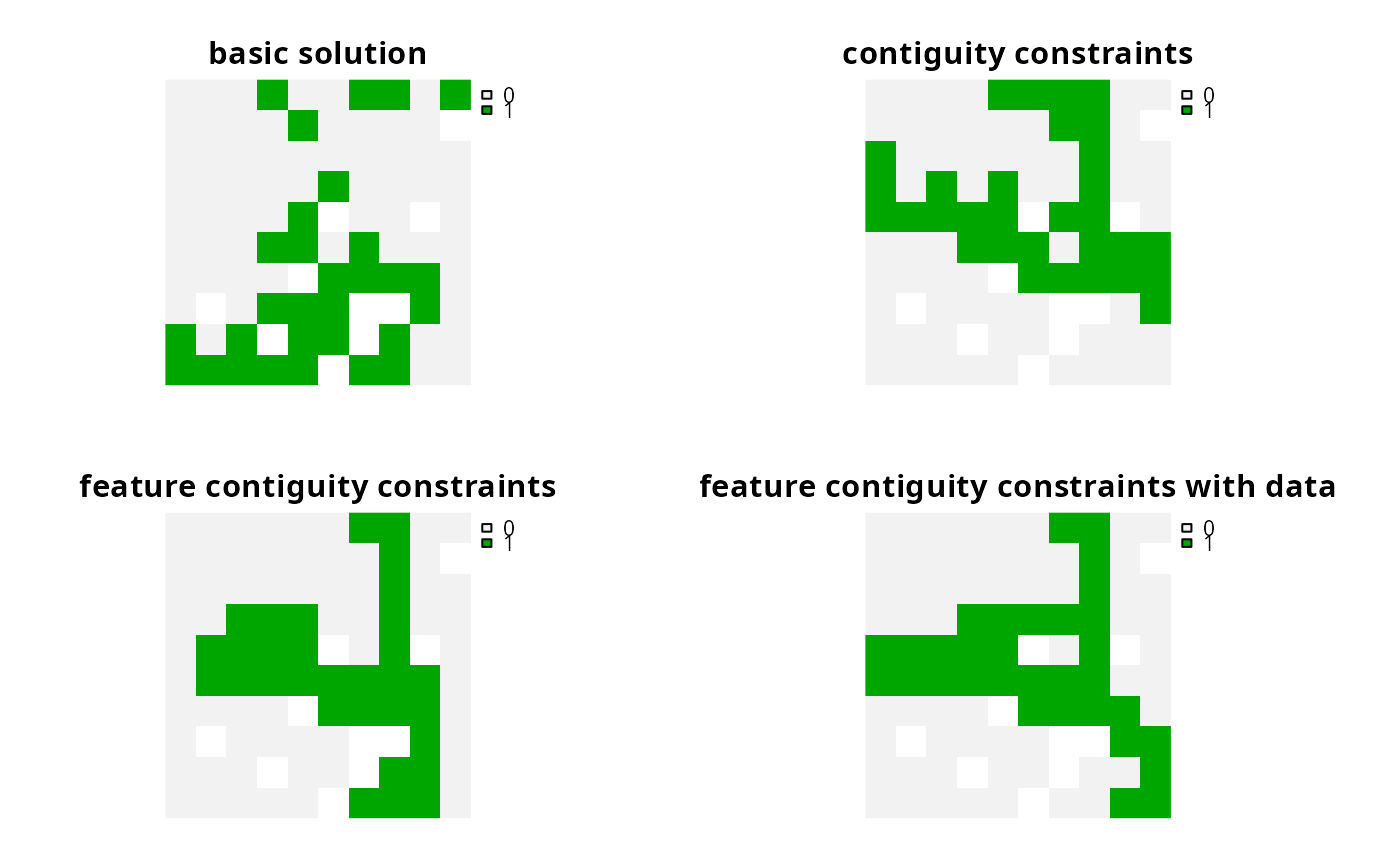
s1 <- c(solve(p1), solve(p2), solve(p3), solve(p4))
names(s1) <- c(
  "basic solution", "contiguity constraints",
  "feature contiguity constraints",
  "feature contiguity constraints with data"
)
# plot solutions
plot(s1, axes = FALSE)


# create minimal problem with multiple zones, and limit the solver to
# 30 seconds to obtain solutions in a feasible period of time
p5 <-
  problem(sim_zones_pu_raster, sim_zones_features) %>%
  add_min_set_objective() %>%
  add_relative_targets(matrix(0.1, ncol = 3, nrow = 5)) %>%
  add_binary_decisions() %>%
  add_default_solver(time_limit = 30, verbose = FALSE)

# create problem with contiguity constraints that specify that the
# planning units used to conserve each feature in different management
# zones must form separate contiguous units
p6 <- p5 %>% add_feature_contiguity_constraints(diag(3))

# create problem with contiguity constraints that specify that the
# planning units used to conserve each feature must form a single
# contiguous unit if the planning units are allocated to zones 1 and 2
# and do not need to form a single contiguous unit if they are allocated
# to zone 3
zm7 <- matrix(0, ncol = 3, nrow = 3)
zm7[seq_len(2), seq_len(2)] <- 1
print(zm7)
#>      [,1] [,2] [,3]
#> [1,]    1    1    0
#> [2,]    1    1    0
#> [3,]    0    0    0
p7 <- p5 %>% add_feature_contiguity_constraints(zm7)

# create problem with contiguity constraints that specify that all of
# the planning units in all three of the zones must conserve first feature
# in a single contiguous unit but the planning units used to conserve the
# remaining features do not need to be contiguous in any way
zm8 <- lapply(
  seq_len(number_of_features(sim_zones_features)),
  function(i) matrix(ifelse(i == 1, 1, 0), ncol = 3, nrow = 3)
)
print(zm8)
#> [[1]]
#>      [,1] [,2] [,3]
#> [1,]    1    1    1
#> [2,]    1    1    1
#> [3,]    1    1    1
#> 
#> [[2]]
#>      [,1] [,2] [,3]
#> [1,]    0    0    0
#> [2,]    0    0    0
#> [3,]    0    0    0
#> 
#> [[3]]
#>      [,1] [,2] [,3]
#> [1,]    0    0    0
#> [2,]    0    0    0
#> [3,]    0    0    0
#> 
#> [[4]]
#>      [,1] [,2] [,3]
#> [1,]    0    0    0
#> [2,]    0    0    0
#> [3,]    0    0    0
#> 
#> [[5]]
#>      [,1] [,2] [,3]
#> [1,]    0    0    0
#> [2,]    0    0    0
#> [3,]    0    0    0
#> 
p8 <- p5 %>% add_feature_contiguity_constraints(zm8)

# solve problems
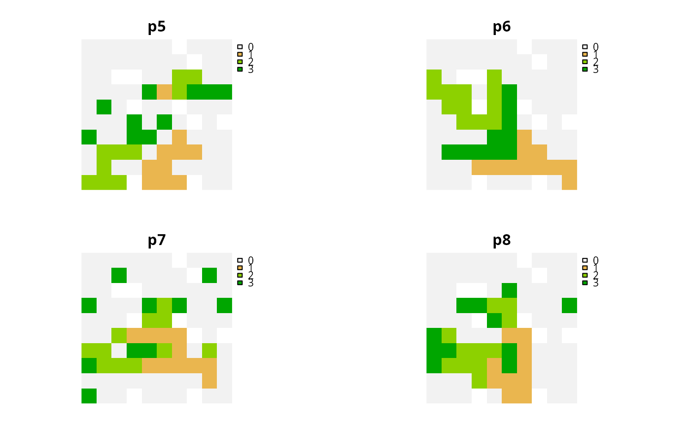
s2 <- lapply(list(p5, p6, p7, p8), solve)
s2 <- terra::rast(lapply(s2, category_layer))
names(s2) <- c("p5", "p6", "p7", "p8")
# plot solutions
plot(s2, axes = FALSE)

# }