Summary
The prioritizr R package uses mixed integer linear programming (MILP) techniques to provide a flexible interface for building and solving conservation planning problems (Rodrigues et al. 2000; Billionnet 2013). It supports a broad range of objectives, constraints, and penalties that can be used to custom-tailor conservation planning problems to the specific needs of a conservation planning exercise. Once built, conservation planning problems can be solved using a variety of commercial and open-source exact algorithm solvers. In contrast to the algorithms conventionally used to solve conservation problems, such as heuristics or simulated annealing (Ball et al. 2009), the exact algorithms used here are guaranteed to find optimal solutions. Furthermore, conservation problems can be constructed to optimize the spatial allocation of different management zones (or actions), meaning that conservation practitioners can identify solutions that benefit multiple stakeholders. Finally, this package has the functionality to read input data formatted for the Marxan conservation planning program (Ball et al. 2009), and find much cheaper solutions in a much shorter period of time than Marxan (Beyer et al. 2016).
Introduction
Systematic conservation planning is a rigorous, repeatable, and structured approach to designing new protected areas that efficiently meet conservation objectives (Margules & Pressey 2000). Historically, conservation decision-making has often evaluated parcels opportunistically as they became available for purchase, donation, or under threat. Although purchasing such areas may improve the status quo, such decisions may not substantially enhance the long-term persistence of target species or communities. Faced with this realization, conservation planners began using decision support tools to help simulate alternative reserve designs over a range of different biodiversity and management goals and, ultimately, guide protected area acquisitions and management actions. Due to the systematic, evidence-based nature of these tools, conservation prioritization can help contribute to a transparent, inclusive, and more defensible decision making process.
A conservation planning exercise typically starts by defining a study area. This study area should encompass all the areas relevant to the decision maker or the hypothesis being tested. The extent of a study area could encompass a few important localities (e.g., Stigner et al. 2016), a single state (e.g., Kirkpatrick 1983), an entire country (Fuller et al. 2010), or the entire planet (Butchart et al. 2015). Next, the study area is divided into a set of discrete areas termed planning units. Each planning unit represents a discrete locality in the study area that can be managed independently of other areas. The general idea is that some combination of the planning units can be selected for conservation actions (e.g., protected area establishment, habitat restoration). Planning units are often created as square or hexagon cells that are sized according to the scale of the conservation actions, and the resolution of the data that underpin the planning exercise (but see Klein et al. 2009).
Cost data (or a surrogate thereof) are needed to inform the prioritization process. Specifically, these cost data describe the relative expenditure associated with managing each planning unit for conservation. For example, if the goal of the conservation planning exercise is to identify priority areas for expanding a local protected area system, then the cost data could represent the physical cost of purchasing the land. Alternatively, if such data are not available, then surrogate data are often used instead (e.g., human population density, opportunity cost of foregone commercial activities, or planning unit size).
Conservation planning exercises also require data on the biodiversity elements that are of conservation interest (termed conservation features). These features could be species (e.g., Neofelis nebulosa, the Clouded Leopard), populations, or habitats (e.g., mangroves or cloud forest). After identifying the set of relevant conservation features for a conservation planning exercise, spatially explicit data need to be obtained for each and every feature to describe their spatial distribution (e.g., habitat suitability data, probability of occurrence data, presence/absence data). This is important to ensure that conservation features are adequately covered (represented) by prioritizations. After assembling all the data, the next step is to define the conservation planning problem.
The prioritizr R package is designed to help you build and solve conservation planning problems. Specifically, prioritizations are generated by formulating a mathematical optimization problem and then solving it to generate a solution. These mathematical optimization problems are formulated using the planning unit data, cost data, and feature data, and with information related to the overarching aim of the prioritization process. In general, the goal of an optimization problem is to minimize (or maximize) an objective function that is calculated using a set of decision variables, subject to a series of constraints to ensure that solution exhibits specific properties. The objective function describes the quantity which we are trying to minimize (e.g., cost of the solution) or maximize (e.g., number of features conserved). The decision variables describe the entities that we can control, and indicate which planning units are selected for conservation management and which are not. The constraints can be thought of as rules that the decision variables need to follow. For example, a commonly used constraint is specifying that the solution must not exceed a certain budget.
A wide variety of approaches have been developed for solving optimization problems. Reserve design problems are frequently solved using simulated annealing (Kirkpatrick et al. 1983) or heuristics (Nicholls & Margules 1993; Moilanen 2007). These methods are conceptually simple and can be applied to a wide variety of optimization problems. However, they do not scale well for large or complex problems (Beyer et al. 2016). Additionally, these methods cannot tell you how close any given solution is to the optimal solution. The prioritizr package uses exact algorithms to efficiently solve conservation planning problems to within a pre-specified optimality gap. In other words, you can specify that you need the optimal solution (i.e., a gap of 0%) and the algorithms will, given enough time, find a solution that meets this criteria. In the past, exact algorithms have been too slow for conservation planning exercises (Pressey et al. 1996). However, improvements over the last decade mean that they are now much faster (Achterberg & Wunderling 2013; Beyer et al. 2016).
In this package, optimization problems are expressed using integer linear programming (ILP) so that they can be solved using (linear) exact algorithm solvers. The general form of an integer programming problem can be expressed in matrix notation using the following equation.
\text{Minimize} \space \boldsymbol{c}^\text{T} \boldsymbol{x} \space \space \text{subject to} \space A\boldsymbol{x} \space \Box \space \boldsymbol{b}
Where x is a vector of decision variables, c and b are vectors of known coefficients, and A is the constraint matrix. The final term specifies a series of structural constants and the \Box symbol is used to indicate that the relational operators for the constraints can be either \geq, =, or \leq. In the context of a conservation planning problem, c could be used to represent the planning unit costs, A could be used to store the data showing the presence / absence (or amount) of each feature in each planning unit, b could be used to represent minimum amount of habitat required for each species in the solution, the \Box could be set to \geq symbols to indicate that the total amount of each feature in the solution must exceed the quantities in b. But there are many other ways of formulating the reserve selection problem (Rodrigues et al. 2000).
A grammar for conservation planning
The prioritizr R package uses a grammar to describe elements
of conservation planning. This means that functions are organized into
verbs that relate to specific concepts. For example, all of the
functions used to specify the primary objective for optimization end
with the _objective suffix (e.g.,
add_min_set_objective() and
add_min_shortfall_objective()). By combining multiple
functions together, they can be used to formulate a complete
conservation planning problem. Specifically, the verbs for formulating
problems are described below.
- Create a new conservation planning problem by specifying the planning units, features, and management zones of conservation interest.
- Add a primary objective to a conservation planning problem (e.g., minimize overall cost).
- Add penalties to a conservation planning problem to penalize solutions according to specific metric (e.g., connectivity).
- Add targets to a conservation planning problem to specify how much of each feature should ideally be represented by solutions.
- Add constraints to a conservation planning problem to ensure that solutions exhibit specific properties (e.g., select specific planning units for protection).
- Add decisions to a conservation planning problem to specify the nature of the decisions in the problem (e.g., binary decisions indicate the planning units should be selected or not selected for management).
- Add a portfolio to a conservation planning problem to specify a methodological approach for generating multiple solutions (e.g., generate multiple solutions by finding 100 solutions within 10% of optimality).
- Add a solver to a conservation problem to specify the optimization software (e.g., Gurobi) for generating solutions and customize the optimization settings (e.g., generate an optimal solution).
After building a conservation planning problem, it can be solved to
generate a prioritization (using the solve() function).
There are also verbs available to help evaluate and interpret solutions.
These verbs are described below.
- Evaluate performance by computing summary statistics (e.g., overall cost, feature representation, or total boundary length).
- Evaluate the relative importance of planning units selected by a solution (e.g., based on irreplaceability).
Workflow
The general workflow when using the prioritizr R package
starts with creating a new conservation planning problem()
object using data. Specifically, the problem() object
should be constructed using data that specify the planning units,
biodiversity features, management zones (if applicable), and costs.
After creating a new problem() object, it can be
customized—by adding objectives, penalties, constraints, and other
information—to build a precise representation of the conservation
planning problem required, and then solved to obtain a solution.
All conservation planning problems require an objective. An objective
specifies the property which is used to compare different feasible
solutions. Simply put, the objective is the property of the solution
which should be maximized or minimized during the optimization process.
For instance, with the minimum set objective (specified using
add_min_set_objective()), we are seeking to minimize the
cost of the solution (similar to Marxan). On the other hand,
with the minimum shortfall objective (specified using
add_min_shortfall_objective()), we are seeking to minimize
the average target shortfall for all features represented in the
solution, subject to a budget.
Many objectives require representation targets (e.g., the minimum set
objective). These targets are a specialized set of constraints that
relate to the total quantity of each feature secured in the solution
(e.g., amount of suitable habitat or number of individuals). In the case
of the minimum set objective (add_min_set_objective()),
targets are used to ensure that solutions must secure a sufficient
quantity of each and every feature. In budget-limited objectives (e.g.,
the minimum shortfall objective;
add_min_shortfall_objective()), candidate solutions do not
have to all meet targets and targets are instead used to specify
trade-offs for representing different features. Targets can be expressed
numerically as the total amount required for a given feature (using
add_absolute_targets()), or as a proportion of the total
amount found in the planning units (using
add_relative_targets()). Note that not all objectives
require targets, and a warning will be thrown if an attempt is made to
add targets to a problem with an objective that does not use them.
Constraints and penalties can be added to a conservation planning
problem to ensure that solutions exhibit a specific property or penalize
solutions which don’t exhibit a specific property (respectively). The
difference between constraints and penalties, strictly speaking, is
constraints are used to rule out potential solutions that don’t exhibit
a specific property. For instance, constraints can be used to ensure
that specific planning units are selected in the solution for
prioritization (using add_locked_in_constraints()) or not
selected in the solution for prioritization (using
add_locked_out_constraints()). On the other hand, penalties
are combined with the objective of a problem, with a penalty factor, and
the overall objective of the problem then becomes to minimize (or
maximize) the primary objective function and the penalty function. For
example, penalties can be added to a problem to penalize solutions that
are excessively fragmented (using
add_boundary_penalties()). These penalties have a
penalty argument that specifies the relative importance of
having spatially clustered solutions. When the argument to
penalty is high, then solutions which are less fragmented
are valued more highly – even if they cost more – and when the argument
to penalty is low, then the solutions which are more
fragmented are valued less highly.
After building a conservation problem, it can then be solved to obtain a solution (or portfolio of solutions if desired). The solution is returned in the same format as the planning unit data used to construct the problem. For instance, this means that if raster data was used to initialize the problem, then the solution will also be output in raster format. This can be very helpful when it comes to interpreting and visualizing solutions because it means that the solution data does not first have to be merged with spatial data before they can be plotted on a map.
Usage
Here we will provide an introduction to using the prioritizr R package to build and solve a conservation planning problem. Please note that we will not discuss conservation planning with multiple zones in this vignette, for more information on working with multiple management zones please see the Management zones tutorial.
First, we will load the prioritizr package.
# load package
library(prioritizr)
Data
Now we will load some built-in data sets that are distributed with the prioritizr R package. This package contains several different planning unit data sets. To provide a comprehensive overview of the different ways that we can initialize a conservation planning problem, we will load each of them.
First, we will load the raster planning unit data
(sim_pu_raster). Here, the planning units are represented
as a single-layer raster object (i.e., a terra::rast()
object) and each pixel corresponds to the spatial extent of each panning
unit. The pixel values correspond to the acquisition costs of each
planning unit.
# load raster planning unit data
sim_pu_raster <- get_sim_pu_raster()

# print data
print(sim_pu_raster)
## class : SpatRaster
## size : 10, 10, 1 (nrow, ncol, nlyr)
## resolution : 0.1, 0.1 (x, y)
## extent : 0, 1, 0, 1 (xmin, xmax, ymin, ymax)
## coord. ref. : WGS 84 / Pseudo-Mercator (EPSG:3857)
## source : sim_pu_raster.tif
## name : layer
## min value : 190.132751
## max value : 215.863846
# plot data
plot(
  sim_pu_raster, main = "Planning unit costs",
  xlim = c(-0.1, 1.1), ylim = c(-0.1, 1.1), axes = FALSE
)
Secondly, we will load one of the spatial vector planning unit data
sets (sim_pu_polygons). Here, each polygon (i.e., feature
using ArcGIS terminology) corresponds to a different planning unit. This
data set has an attribute table that contains additional information
about each polygon. Namely, the cost field (column) in the
attribute table contains the acquisition cost for each planning
unit.
# load polygon planning unit data
sim_pu_polygons <- get_sim_pu_polygons()

# print data
print(sim_pu_polygons)
## Simple feature collection with 90 features and 3 fields
## Geometry type: POLYGON
## Dimension: XY
## Bounding box: xmin: 0 ymin: 0 xmax: 1 ymax: 1
## Projected CRS: WGS 84 / Pseudo-Mercator
## # A tibble: 90 × 4
## cost locked_in locked_out geom
## * <dbl> <lgl> <lgl> <POLYGON [m]>
## 1 216. FALSE FALSE ((0 1, 0.1 1, 0.1 0.9, 0 0.9, 0 1))
## 2 213. FALSE FALSE ((0.1 1, 0.2 1, 0.2 0.9, 0.1 0.9, 0.1 1))
## 3 207. FALSE FALSE ((0.2 1, 0.3 1, 0.3 0.9, 0.2 0.9, 0.2 1))
## 4 209. FALSE TRUE ((0.3 1, 0.4 1, 0.4 0.9, 0.3 0.9, 0.3 1))
## 5 214. FALSE FALSE ((0.4 1, 0.5 1, 0.5 0.9, 0.4 0.9, 0.4 1))
## 6 214. FALSE FALSE ((0.5 1, 0.6 1, 0.6 0.9, 0.5 0.9, 0.5 1))
## 7 210. FALSE FALSE ((0.6 1, 0.7 1, 0.7 0.9, 0.6 0.9, 0.6 1))
## 8 211. FALSE TRUE ((0.7 1, 0.8 1, 0.8 0.9, 0.7 0.9, 0.7 1))
## 9 210. FALSE FALSE ((0.8 1, 0.9 1, 0.9 0.9, 0.8 0.9, 0.8 1))
## 10 204. FALSE FALSE ((0.9 1, 1 1, 1 0.9, 0.9 0.9, 0.9 1))
## # ℹ 80 more rows
# plot the planning units, and color them according to cost values
plot(sim_pu_polygons[, "cost"])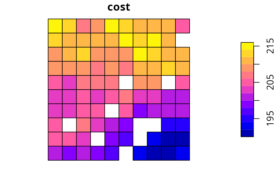
Thirdly, we will load some planning unit data stored in tabular
format (i.e., data.frame format). For those familiar with
Marxan or dealing with very large conservation planning
problems (> 10 million planning units), it may be useful to work with
data in this format because it does not contain any spatial information
which will reduce computational burden. When using tabular data to
initialize conservation planning problems, the data must follow the
conventions used by Marxan. Specifically, each row in the
planning unit table must correspond to a different planning unit. The
table must also have an “id” column to provide a unique integer
identifier for each planning unit, and it must also have a column that
indicates the cost of each planning unit. For more information, please
see the official Marxan
documentation.
# specify file path for planning unit data
pu_path <- system.file("extdata/marxan/input/pu.dat", package = "prioritizr")

# load in the tabular planning unit data
pu_dat <- vroom::vroom(pu_path)
## Rows: 1751 Columns: 5
## ── Column specification ────────────────────────────────────────────────────────
## Delimiter: ","
## dbl (5): id, cost, status, xloc, yloc
##
## ℹ Use `spec()` to retrieve the full column specification for this data.
## ℹ Specify the column types or set `show_col_types = FALSE` to quiet this message.
# preview first six rows of the tabular planning unit data
# note that it has some extra columns other than id and cost as per the
# Marxan format
head(pu_dat)
## # A tibble: 6 × 5
## id cost status xloc yloc
## <dbl> <dbl> <dbl> <dbl> <dbl>
## 1 3 0 0 1116623. -4493479.
## 2 30 7527. 3 1110623. -4496943.
## 3 56 37349. 0 1092623. -4500408.
## 4 58 16959. 0 1116623. -4500408.
## 5 84 34220. 0 1098623. -4503872.
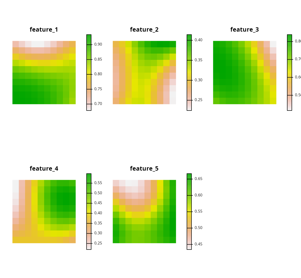
## 6 85 178908. 0 1110623. -4503872.Finally, we will load data showing the spatial distribution of the
conservation features. Our conservation features
(sim_features) are represented as a multi-layer raster
object (i.e., a terra::rast() object), where each layer
corresponds to a different feature. The pixel values in each layer
correspond to the amount of suitable habitat available in a given
planning unit. Note that our planning unit and our feature data have
exactly the same spatial properties (i.e., resolution, extent,
coordinate reference system) so their pixels line up perfectly.
# load feature data
sim_features <- get_sim_features()

# plot the distribution of suitable habitat for each feature
plot(
  sim_features, nr = 2,
  axes = FALSE, xlim = c(-0.1, 1.1), ylim = c(-0.1, 1.1)
)
Initialize a problem
After having loaded our planning unit and feature data, we will now
try initializing some conservation planning problems. There are a lot of
different ways to initialize a conservation planning problem, so here we
will just showcase a few of the more commonly used methods. For an
exhaustive description of all the ways you can initialize a conservation
problem, see the help file for the problem() function.
First off, we will initialize a conservation planning problem using the
raster data.
## A conservation problem (<ConservationProblem>)
## ├•data
## │├•features:    "feature_1", "feature_2", "feature_3", … (5 total)
## │└•planning units:
## │ ├•data:       <SpatRaster> (90 total)
## │ ├•costs:      continuous values (between 190.1328 and 215.8638)
## │ ├•extent:     0, 0, 1, 1 (xmin, ymin, xmax, ymax)
## │ └•CRS:        WGS 84 / Pseudo-Mercator (projected)
## ├•formulation
## │├•objective:   none specified
## │├•penalties:   none specified
## │├•features:
## ││├•targets:    none specified
## ││└•weights:    none specified
## │├•constraints: none specified
## │└•decisions:   binary decision
## └•optimization
##  ├•portfolio:   single portfolio
##  └•solver:      gurobi solver (`gap` = 0.1, `time_limit` = 2147483647, …)
## # ℹ Use `summary(...)` to see further details.
# print number of planning units
number_of_planning_units(p1)
## [1] 90
# print number of features
number_of_features(p1)
## [1] 5Generally, we recommend initializing problems using raster data where
possible. This is because the problem() function needs to
calculate the amount of each feature in each planning unit, and by
providing both the planning unit and feature data in raster format with
the same spatial resolution, extents, and coordinate systems, this means
that the problem() function does not need to do any
geoprocessing behind the scenes. But sometimes we can’t use raster
planning unit data, because our planning units aren’t equal-sized grid
cells. So, below is an example showing how we can initialize a
conservation planning problem using planning units that are formatted as
spatial vector data. Note that we could reduce run-time by pre-computing
the amount of each feature in each planning unit and storing the data in
the attribute table (e.g., by performing zonal statistics with
R or ESRI ArcGIS), and then passing in the names of
the columns as an argument to the problem() function (see
Examples section for problem() for details).
# create problem with spatial vector data
# note that we have to specify which column in the attribute table contains
# the cost data
p2 <- problem(sim_pu_polygons, sim_features, cost_column = "cost")

# print problem
print(p2)
## A conservation problem (<ConservationProblem>)
## ├•data
## │├•features: "feature_1", "feature_2", "feature_3", … (5 total)
## │└•planning units:
## │ ├•data: <sf> (90 total)
## │ ├•costs: continuous values (between 190.1328 and 215.8638)
## │ ├•extent: 0, 0, 1, 1 (xmin, ymin, xmax, ymax)
## │ └•CRS: WGS 84 / Pseudo-Mercator (projected)
## ├•formulation
## │├•objective: none specified
## │├•penalties: none specified
## │├•features:
## ││├•targets: none specified
## ││└•weights: none specified
## │├•constraints: none specified
## │└•decisions: binary decision
## └•optimization
## ├•portfolio: single portfolio
## └•solver: gurobi solver (`gap` = 0.1, `time_limit` = 2147483647, …)
## # ℹ Use `summary(...)` to see further details.We can also initialize a conservation planning problem using tabular
planning unit data (i.e., data.frame format). Since the
tabular planning unit data does not contain any spatial information, we
also have to provide the feature data in tabular format (i.e.,
data.frame format) and data showing the amount of each
feature in each planning unit in tabular format (i.e.,
data.frame format). The feature data must have an “id”
column containing a unique integer identifier for each feature, and the
planning unit by feature data must contain the following three columns:
pu corresponding to the planning unit identifiers,
species corresponding to the feature identifiers, and
amount showing the amount of a given feature in a given
planning unit.
# set file path for feature data
spec_path <- system.file(
  "extdata/marxan/input/spec.dat", package = "prioritizr"
)

# load in feature data
spec_dat <- vroom::vroom(spec_path)
## Rows: 17 Columns: 4
## ── Column specification ────────────────────────────────────────────────────────
## Delimiter: ","
## chr (1): name
## dbl (3): id, prop, spf
##
## ℹ Use `spec()` to retrieve the full column specification for this data.
## ℹ Specify the column types or set `show_col_types = FALSE` to quiet this message.
# print first six rows of the data
# note that it contains extra columns
head(spec_dat)
## # A tibble: 6 × 4
## id prop spf name
## <dbl> <dbl> <dbl> <chr>
## 1 10 0.3 1 bird1
## 2 11 0.3 1 nvis2
## 3 12 0.3 1 nvis8
## 4 13 0.3 1 nvis9
## 5 14 0.3 1 nvis14
## 6 15 0.3 1 nvis20
# set file path for planning unit vs. feature data
puvspr_path <- system.file(
  "extdata/marxan/input/puvspr.dat", package = "prioritizr"
)

# load in planning unit vs feature data
puvspr_dat <- vroom::vroom(puvspr_path)
## Rows: 4662 Columns: 3
## ── Column specification ────────────────────────────────────────────────────────
## Delimiter: ","
## dbl (3): species, pu, amount
##
## ℹ Use `spec()` to retrieve the full column specification for this data.
## ℹ Specify the column types or set `show_col_types = FALSE` to quiet this message.
# print first six rows of the data
head(puvspr_dat)
## # A tibble: 6 × 3
## species pu amount
## <dbl> <dbl> <dbl>
## 1 26 56 120.
## 2 26 58 45.2
## 3 26 84 68.0
## 4 26 85 9.74
## 5 26 86 7.80
## 6 26 111 478.
# create problem
p3 <- problem(pu_dat, spec_dat, cost_column = "cost", rij = puvspr_dat)

# print problem
print(p3)
## A conservation problem (<ConservationProblem>)
## ├•data
## │├•features: "bird1", "nvis2", "nvis8", "nvis9", … (17 total)
## │└•planning units:
## │ ├•data: <spec_tbl_df> (1751 total)
## │ ├•costs: continuous values (between 0 and 415692.2)
## │ ├•extent: NA
## │ └•CRS: NA
## ├•formulation
## │├•objective: none specified
## │├•penalties: none specified
## │├•features:
## ││├•targets: none specified
## ││└•weights: none specified
## │├•constraints: none specified
## │└•decisions: binary decision
## └•optimization
## ├•portfolio: single portfolio
## └•solver: gurobi solver (`gap` = 0.1, `time_limit` = 2147483647, …)
## # ℹ Use `summary(...)` to see further details.For more information on initializing problems, please see the help
page for the problem() function (which you can open by
entering the code: ?problem). Now that we have initialized
a conservation planning problem, we will show you how you can customize
it to suit the exact needs of your conservation planning scenario.
Although we initialized the conservation planning problems using several
different methods, moving forward, we will only use raster-based
planning unit data to keep things simple.
Add an objective
The next step is to add a primary objective to the problem. A problem objective is used to specify the primary goal of the problem (i.e., the quantity that is to be maximized or minimized). All conservation planning problems involve minimizing or maximizing some kind of objective. For instance, we might require a solution that conserves enough habitat for each species while minimizing the overall cost of the reserve network. Alternatively, we might require a solution that maximizes the number of conserved species while ensuring that the cost of the reserve network does not exceed the budget. Please note that objectives are added in the same way regardless of the type of data used to initialize the problem. The following objectives are available.
- Minimum set objective: Minimize the cost of the solution whilst ensuring that all targets are met (Rodrigues et al. 2000). This objective is similar to that used in Marxan (Ball et al. 2009). For example, we can add a minimum set objective to a problem using the following code.
# create a new problem that has the minimum set objective
p3 <-
  problem(sim_pu_raster, sim_features) %>%
  add_min_set_objective()

# print problem
print(p3)
## A conservation problem (<ConservationProblem>)
## ├•data
## │├•features: "feature_1", "feature_2", "feature_3", … (5 total)
## │└•planning units:
## │ ├•data: <SpatRaster> (90 total)
## │ ├•costs: continuous values (between 190.1328 and 215.8638)
## │ ├•extent: 0, 0, 1, 1 (xmin, ymin, xmax, ymax)
## │ └•CRS: WGS 84 / Pseudo-Mercator (projected)
## ├•formulation
## │├•objective: minimum set objective
## │├•penalties: none specified
## │├•features:
## ││├•targets: none specified
## ││└•weights: none specified
## │├•constraints: none specified
## │└•decisions: binary decision
## └•optimization
## ├•portfolio: single portfolio
## └•solver: gurobi solver (`gap` = 0.1, `time_limit` = 2147483647, …)
## # ℹ Use `summary(...)` to see further details.- Maximum cover objective: Represent at least one instance of as many features as possible within a given budget (Church et al. 1996).
# create a new problem that has the maximum coverage objective and a budget
# of 5000
p4 <-
  problem(sim_pu_raster, sim_features) %>%
  add_max_cover_objective(5000)

# print problem
print(p4)
## A conservation problem (<ConservationProblem>)
## ├•data
## │├•features: "feature_1", "feature_2", "feature_3", … (5 total)
## │└•planning units:
## │ ├•data: <SpatRaster> (90 total)
## │ ├•costs: continuous values (between 190.1328 and 215.8638)
## │ ├•extent: 0, 0, 1, 1 (xmin, ymin, xmax, ymax)
## │ └•CRS: WGS 84 / Pseudo-Mercator (projected)
## ├•formulation
## │├•objective: maximum coverage objective (`budget` = 5000)
## │├•penalties: none specified
## │├•features:
## ││├•targets: none specified
## ││└•weights: none specified
## │├•constraints: none specified
## │└•decisions: binary decision
## └•optimization
## ├•portfolio: single portfolio
## └•solver: gurobi solver (`gap` = 0.1, `time_limit` = 2147483647, …)
## # ℹ Use `summary(...)` to see further details.- Maximum number of targets met objective: Fulfill as many targets as possible while ensuring that the cost of the solution does not exceed a budget (inspired by Cabeza & Moilanen 2001). Note that this objective does not value the partial fulfillment of targets. This objective is similar to the maximum cover objective except that we have the option of later specifying targets for each feature. In practice, this objective is more useful than the maximum cover objective because features often require a certain amount of area for them to persist and simply capturing a single instance of habitat for each feature is generally unlikely to enhance their long-term persistence.
# create a new problem that has the maximum number of targets met objective and
# a budget of 5000
p5 <-
  problem(sim_pu_raster, sim_features) %>%
  add_max_n_targets_met_objective(budget = 5000)

# print problem
print(p5)
## A conservation problem (<ConservationProblem>)
## ├•data
## │├•features: "feature_1", "feature_2", "feature_3", … (5 total)
## │└•planning units:
## │ ├•data: <SpatRaster> (90 total)
## │ ├•costs: continuous values (between 190.1328 and 215.8638)
## │ ├•extent: 0, 0, 1, 1 (xmin, ymin, xmax, ymax)
## │ └•CRS: WGS 84 / Pseudo-Mercator (projected)
## ├•formulation
## │├•objective: maximum number targets met objective (`budget` = 5000)
## │├•penalties: none specified
## │├•features:
## ││├•targets: none specified
## ││└•weights: none specified
## │├•constraints: none specified
## │└•decisions: binary decision
## └•optimization
## ├•portfolio: single portfolio
## └•solver: gurobi solver (`gap` = 0.1, `time_limit` = 2147483647, …)
## # ℹ Use `summary(...)` to see further details.-
Minimum shortfall objective: Minimize the overall
(weighted sum) shortfall for as many targets as possible while ensuring
that the cost of the solution does not exceed a budget. In general, we
recommend using this objective for budget-limited planning exercises.
Although the maximum number of targets met objective
(
add_max_n_targets_met_objective()) will often produce solutions that have unspent (or left-over) funding, this objective does not have this limitation because it values the partial fulfillment of targets.
# create a new problem that has the minimum shortfall objective and a budget
# of 5000
p6 <-
  problem(sim_pu_raster, sim_features) %>%
  add_min_shortfall_objective(budget = 5000)

# print problem
print(p6)
## A conservation problem (<ConservationProblem>)
## ├•data
## │├•features: "feature_1", "feature_2", "feature_3", … (5 total)
## │└•planning units:
## │ ├•data: <SpatRaster> (90 total)
## │ ├•costs: continuous values (between 190.1328 and 215.8638)
## │ ├•extent: 0, 0, 1, 1 (xmin, ymin, xmax, ymax)
## │ └•CRS: WGS 84 / Pseudo-Mercator (projected)
## ├•formulation
## │├•objective: minimum shortfall objective (`budget` = 5000)
## │├•penalties: none specified
## │├•features:
## ││├•targets: none specified
## ││└•weights: none specified
## │├•constraints: none specified
## │└•decisions: binary decision
## └•optimization
## ├•portfolio: single portfolio
## └•solver: gurobi solver (`gap` = 0.1, `time_limit` = 2147483647, …)
## # ℹ Use `summary(...)` to see further details.- Minimum largest shortfall objective: Minimize the largest (maximum) shortfall while ensuring that the cost of the solution does not exceed a budget. In practice, this objective useful when the minimum shortfall objective returns solutions that focus too much on representing a small number of features (e.g., because they occur in much cheaper planning units), and solutions are needed to spread conservation effort out more evenly among all features—even if it means that all features will have (relatively) poor representation.
# create a new problem that has the minimum largest shortfall objective and a
# budget of 5000
p7 <-
  problem(sim_pu_raster, sim_features) %>%
  add_min_largest_shortfall_objective(budget = 5000)

# print problem
print(p7)
## A conservation problem (<ConservationProblem>)
## ├•data
## │├•features: "feature_1", "feature_2", "feature_3", … (5 total)
## │└•planning units:
## │ ├•data: <SpatRaster> (90 total)
## │ ├•costs: continuous values (between 190.1328 and 215.8638)
## │ ├•extent: 0, 0, 1, 1 (xmin, ymin, xmax, ymax)
## │ └•CRS: WGS 84 / Pseudo-Mercator (projected)
## ├•formulation
## │├•objective: minimum largest shortfall objective (`budget` = 5000)
## │├•penalties: none specified
## │├•features:
## ││├•targets: none specified
## ││└•weights: none specified
## │├•constraints: none specified
## │└•decisions: binary decision
## └•optimization
## ├•portfolio: single portfolio
## └•solver: gurobi solver (`gap` = 0.1, `time_limit` = 2147483647, …)
## # ℹ Use `summary(...)` to see further details.-
Maximum phylogenetic diversity objective: Maximize
the phylogenetic diversity of the features represented in the solution
subject to a budget (inspired by Faith 1992;
Rodrigues & Gaston 2002). This objective is similar to the
maximum number of targets met objective
(
add_max_n_targets_met()) except that emphasis is placed on protecting features which are associated with a diverse range of evolutionary histories. The package contains a simulated phylogeny that can be used with the simulated feature data (sim_phylogny).
# load simulated phylogeny data
sim_phylogeny <- get_sim_phylogeny()

# create a new problem that has the maximum phylogenetic diversity
# objective and a budget of 5000
p8 <-
  problem(sim_pu_raster, sim_features) %>%
  add_max_phylo_div_objective(budget = 5000, tree = sim_phylogeny)

# print problem
print(p8)
## A conservation problem (<ConservationProblem>)
## ├•data
## │├•features: "feature_1", "feature_2", "feature_3", … (5 total)
## │└•planning units:
## │ ├•data: <SpatRaster> (90 total)
## │ ├•costs: continuous values (between 190.1328 and 215.8638)
## │ ├•extent: 0, 0, 1, 1 (xmin, ymin, xmax, ymax)
## │ └•CRS: WGS 84 / Pseudo-Mercator (projected)
## ├•formulation
## │├•objective: phylogenetic diversity objective (`budget` = 5000, …)
## │├•penalties: none specified
## │├•features:
## ││├•targets: none specified
## ││└•weights: none specified
## │├•constraints: none specified
## │└•decisions: binary decision
## └•optimization
## ├•portfolio: single portfolio
## └•solver: gurobi solver (`gap` = 0.1, `time_limit` = 2147483647, …)
## # ℹ Use `summary(...)` to see further details.- Maximum phylogenetic endemism objective: Maximize the phylogenetic endemism of the features represented in the solution subject to a budget (inspired by Faith 1992; Rodrigues & Gaston 2002; Rosauer et al. 2009). This objective is similar to the maximum phylogenetic diversity except that emphasis is placed on conserving features that are associated with geographically restricted periods of evolutionary history rather than a diverse range of evolutionary histories.
# load simulated phylogeny data
sim_phylogeny <- get_sim_phylogeny()

# create a new problem that has the maximum phylogenetic diversity
# objective and a budget of 5000
p9 <-
  problem(sim_pu_raster, sim_features) %>%
  add_max_phylo_end_objective(budget = 5000, tree = sim_phylogeny)

# print problem
print(p9)
## A conservation problem (<ConservationProblem>)
## ├•data
## │├•features: "feature_1", "feature_2", "feature_3", … (5 total)
## │└•planning units:
## │ ├•data: <SpatRaster> (90 total)
## │ ├•costs: continuous values (between 190.1328 and 215.8638)
## │ ├•extent: 0, 0, 1, 1 (xmin, ymin, xmax, ymax)
## │ └•CRS: WGS 84 / Pseudo-Mercator (projected)
## ├•formulation
## │├•objective: phylogenetic endemism objective (`budget` = 5000, …)
## │├•penalties: none specified
## │├•features:
## ││├•targets: none specified
## ││└•weights: none specified
## │├•constraints: none specified
## │└•decisions: binary decision
## └•optimization
## ├•portfolio: single portfolio
## └•solver: gurobi solver (`gap` = 0.1, `time_limit` = 2147483647, …)
## # ℹ Use `summary(...)` to see further details.- Maximum weighted sum objective: Maximize the weighted sum of the features represented by the solution as much as possible without exceeding a budget. This objective is functionally equivalent to selecting the planning units with the greatest amounts of each feature (e.g., weighted species richness). Generally, we don’t encourage the use of this objective because it will only rarely identify complementary solutions – solutions which adequately conserve a range of different features – except perhaps to explore trade-offs or provide a baseline solution with which to compare other solutions.
# create a new problem that has the maximum weighted sum objective and a budget
# of 5000
p10 <-
  problem(sim_pu_raster, sim_features) %>%
  add_max_wtd_sum_objective(budget = 5000)
## ℹ `add_max_wtd_sum_objective()` has severe limitations - use
## with caution.
# print problem
print(p10)
## A conservation problem (<ConservationProblem>)
## ├•data
## │├•features: "feature_1", "feature_2", "feature_3", … (5 total)
## │└•planning units:
## │ ├•data: <SpatRaster> (90 total)
## │ ├•costs: continuous values (between 190.1328 and 215.8638)
## │ ├•extent: 0, 0, 1, 1 (xmin, ymin, xmax, ymax)
## │ └•CRS: WGS 84 / Pseudo-Mercator (projected)
## ├•formulation
## │├•objective: maximum weighted sum objective (`budget` = 5000)
## │├•penalties: none specified
## │├•features:
## ││├•targets: none specified
## ││└•weights: none specified
## │├•constraints: none specified
## │└•decisions: binary decision
## └•optimization
## ├•portfolio: single portfolio
## └•solver: gurobi solver (`gap` = 0.1, `time_limit` = 2147483647, …)
## # ℹ Use `summary(...)` to see further details.- Minimum penalties objective: Minimize only the penalties added to the problem, whilst ensuring that al targets are met and the cost of the solution does not exceed a budget. This objective is useful when using a hierarchical approach for multi-objective optimization.
# create a new problem that has the minimum penalties objective and a budget
# of 5000
p11 <-
  problem(sim_pu_raster, sim_features) %>%
  add_min_penalties_objective(budget = 5000)

# print problem
print(p11)
## A conservation problem (<ConservationProblem>)
## ├•data
## │├•features: "feature_1", "feature_2", "feature_3", … (5 total)
## │└•planning units:
## │ ├•data: <SpatRaster> (90 total)
## │ ├•costs: continuous values (between 190.1328 and 215.8638)
## │ ├•extent: 0, 0, 1, 1 (xmin, ymin, xmax, ymax)
## │ └•CRS: WGS 84 / Pseudo-Mercator (projected)
## ├•formulation
## │├•objective: minimum penalties objective (`budget` = 5000)
## │├•penalties: none specified
## │├•features:
## ││├•targets: none specified
## ││└•weights: none specified
## │├•constraints: none specified
## │└•decisions: binary decision
## └•optimization
## ├•portfolio: single portfolio
## └•solver: gurobi solver (`gap` = 0.1, `time_limit` = 2147483647, …)
## # ℹ Use `summary(...)` to see further details.Add targets
Most conservation planning problems require targets. Targets are used to specify the minimum amount or proportion of a feature’s distribution that needs to be represented (in other words, covered) by the solution. For example, we may want to develop a reserve network that will secure 20% of the distribution for each feature for minimal cost. As with the functions for specifying the objective of a problem, if we try adding multiple targets to a problem, only the most recently added set of targets are used. The following methods are available for specifying targets.
- Absolute targets: Targets are expressed as the total amount of each feature in the study area that need to be secured. For example, if we had binary feature data that showed the absence or presence of suitable habitat across the study area, we could set an absolute target of 5 to mean that we require 5 planning units with suitable habitat in the solution.
# create a problem with targets which specify that the solution must conserve
# a sum total of 3 units of suitable habitat for each feature
p12 <-
  problem(sim_pu_raster, sim_features) %>%
  add_min_set_objective() %>%
  add_absolute_targets(3)

# print problem
print(p12)
## A conservation problem (<ConservationProblem>)
## ├•data
## │├•features: "feature_1", "feature_2", "feature_3", … (5 total)
## │└•planning units:
## │ ├•data: <SpatRaster> (90 total)
## │ ├•costs: continuous values (between 190.1328 and 215.8638)
## │ ├•extent: 0, 0, 1, 1 (xmin, ymin, xmax, ymax)
## │ └•CRS: WGS 84 / Pseudo-Mercator (projected)
## ├•formulation
## │├•objective: minimum set objective
## │├•penalties: none specified
## │├•features:
## ││├•targets: absolute targets (all equal to 3)
## ││└•weights: none specified
## │├•constraints: none specified
## │└•decisions: binary decision
## └•optimization
## ├•portfolio: single portfolio
## └•solver: gurobi solver (`gap` = 0.1, `time_limit` = 2147483647, …)
## # ℹ Use `summary(...)` to see further details.- Relative targets: Targets are set as a proportion (between 0 and 1) of the total amount of each feature in the study area. For example, if we had binary feature data and the feature occupied a total of 20 planning units in the study area, we could set a relative target of 0.5 (i.e., 50%) to specify that the solution must secure 10 planning units for the feature. We could alternatively specify an absolute target of 10 to achieve the same result, but sometimes proportions are easier to work with.
# create a problem with the minimum set objective and relative targets of 10%
# for each feature
p13 <-
  problem(sim_pu_raster, sim_features) %>%
  add_min_set_objective() %>%
  add_relative_targets(0.1)

# print problem
print(p13)
## A conservation problem (<ConservationProblem>)
## ├•data
## │├•features: "feature_1", "feature_2", "feature_3", … (5 total)
## │└•planning units:
## │ ├•data: <SpatRaster> (90 total)
## │ ├•costs: continuous values (between 190.1328 and 215.8638)
## │ ├•extent: 0, 0, 1, 1 (xmin, ymin, xmax, ymax)
## │ └•CRS: WGS 84 / Pseudo-Mercator (projected)
## ├•formulation
## │├•objective: minimum set objective
## │├•penalties: none specified
## │├•features:
## ││├•targets: relative targets (all equal to 0.1)
## ││└•weights: none specified
## │├•constraints: none specified
## │└•decisions: binary decision
## └•optimization
## ├•portfolio: single portfolio
## └•solver: gurobi solver (`gap` = 0.1, `time_limit` = 2147483647, …)
## # ℹ Use `summary(...)` to see further details.
# create a problem with targets which specify that we need 10% of the habitat
# for the first feature, 15 % for the second feature, 20 % for the third feature
# 25 % for the fourth feature and 30 % of the habitat for the fifth feature
targets <- c(0.1, 0.15, 0.2, 0.25, 0.3)
p14 <-
  problem(sim_pu_raster, sim_features) %>%
  add_min_set_objective() %>%
  add_relative_targets(targets)

# print problem
print(p14)
## A conservation problem (<ConservationProblem>)
## ├•data
## │├•features: "feature_1", "feature_2", "feature_3", … (5 total)
## │└•planning units:
## │ ├•data: <SpatRaster> (90 total)
## │ ├•costs: continuous values (between 190.1328 and 215.8638)
## │ ├•extent: 0, 0, 1, 1 (xmin, ymin, xmax, ymax)
## │ └•CRS: WGS 84 / Pseudo-Mercator (projected)
## ├•formulation
## │├•objective: minimum set objective
## │├•penalties: none specified
## │├•features:
## ││├•targets: relative targets (between 0.1 and 0.3)
## ││└•weights: none specified
## │├•constraints: none specified
## │└•decisions: binary decision
## └•optimization
## ├•portfolio: single portfolio
## └•solver: gurobi solver (`gap` = 0.1, `time_limit` = 2147483647, …)
## # ℹ Use `summary(...)` to see further details.-
Automatic targets: Targets are set following a
particular target setting method. This is provided as a convenient
interface for setting targets based on published methodologies. Target
setting methods can be specified using the following functions:
spec_absolute_targets(),spec_area_targets(),spec_relative_targets(),spec_interp_absolute_targets(),spec_interp_area_targets(),spec_duran_targets(),spec_jung_targets(),spec_polak_targets(),spec_pop_size_targets(),spec_rl_ecosystem_targets(),spec_rl_species_targets(),spec_rodrigues_targets(),spec_rule_targets(),spec_sreekar_targets(),spec_ward_targets(),spec_watson_targets(), andspec_wilson_targets(). Additionally, if a targets should be calculated based on the maximum or minimum thresholds obtained from multiple target setting methods, then thespec_max_targets()andspec_min_targets()functions can be used. Note that this is designed for problems that pertain to a single management zone.
# create a problem with the minimum set objective and relative targets of 10%
# for each feature
p15 <-
  problem(sim_pu_raster, sim_features) %>%
  add_min_set_objective() %>%
  add_auto_targets(method = spec_relative_targets(0.1))

# print problem
print(p15)
## A conservation problem (<ConservationProblem>)
## ├•data
## │├•features: "feature_1", "feature_2", "feature_3", … (5 total)
## │└•planning units:
## │ ├•data: <SpatRaster> (90 total)
## │ ├•costs: continuous values (between 190.1328 and 215.8638)
## │ ├•extent: 0, 0, 1, 1 (xmin, ymin, xmax, ymax)
## │ └•CRS: WGS 84 / Pseudo-Mercator (projected)
## ├•formulation
## │├•objective: minimum set objective
## │├•penalties: none specified
## │├•features:
## ││├•targets: Relative targets (relative values all equal to 0.1)
## ││└•weights: none specified
## │├•constraints: none specified
## │└•decisions: binary decision
## └•optimization
## ├•portfolio: single portfolio
## └•solver: gurobi solver (`gap` = 0.1, `time_limit` = 2147483647, …)
## # ℹ Use `summary(...)` to see further details.-
Group targets: Targets are set for groups of
features following a user-specified target setting method. This is
provided as a convenient alternative for
add_auto_targets()when different target setting methods should be used for different features (e.g., when using different methods for features that correspond to species and habitat types). Similar toadd_auto_targets(), Target setting methods can be specified using the following functions:spec_absolute_targets(),spec_area_targets(),spec_relative_targets(),spec_interp_absolute_targets(),spec_interp_area_targets(),spec_duran_targets(),spec_jung_targets(),spec_polak_targets(),spec_pop_size_targets(),spec_rl_ecosystem_targets(),spec_rl_species_targets(),spec_rodrigues_targets(),spec_rule_targets(),spec_ward_targets(),spec_watson_targets(), andspec_wilson_targets(). Additionally, if a targets should be calculated based on the maximum or minimum thresholds obtained from multiple target setting methods, then thespec_max_targets()andspec_min_targets()functions can be used. Note that this is designed for problems that pertain to a single management zone.
# create a problem with the minimum set objective and relative targets of 10%
# for the first three features (assigned to the group a) and 20% targets
# for the last two features (assigned to the group b)
p16 <-
  problem(sim_pu_raster, sim_features) %>%
  add_min_set_objective() %>%
  add_group_targets(
    groups = c("a", "a", "a", "b", "b"),
    method = list(
      "a" = spec_relative_targets(0.1),
      "b" = spec_relative_targets(0.2)
    )
  )

# print problem
print(p16)
## A conservation problem (<ConservationProblem>)
## ├•data
## │├•features: "feature_1", "feature_2", "feature_3", … (5 total)
## │└•planning units:
## │ ├•data: <SpatRaster> (90 total)
## │ ├•costs: continuous values (between 190.1328 and 215.8638)
## │ ├•extent: 0, 0, 1, 1 (xmin, ymin, xmax, ymax)
## │ └•CRS: WGS 84 / Pseudo-Mercator (projected)
## ├•formulation
## │├•objective: minimum set objective
## │├•penalties: none specified
## │├•features:
## ││├•targets: Relative targets (relative values between 0.1 and 0.2)
## ││└•weights: none specified
## │├•constraints: none specified
## │└•decisions: binary decision
## └•optimization
## ├•portfolio: single portfolio
## └•solver: gurobi solver (`gap` = 0.1, `time_limit` = 2147483647, …)
## # ℹ Use `summary(...)` to see further details.- Manual targets: Targets are set by manually specifying all the required information for each target. This is only really recommended for advanced users or problems that involve multiple management zones. See Management zones tutorial for more information on these targets.
# create a data frame with the following targets:
# a relative target of 10% for the second feature,
# an absolute target of 5 for the third feature,
# and an absolute target of 100 for the fifth feature that specifies the
# maximum level of representation (i.e., not the minimum level, unlike all
# targets discussed previously)
man_targets <- data.frame(
  feature = c("feature_2", "feature_3", "feature_5"),
  type = c("relative", "absolute", "absolute"),
  sense = c(">=", ">=", "<="),
  target = c(0.1, 5, 100)
)
print(man_targets)
## feature type sense target
## 1 feature_2 relative >= 0.1
## 2 feature_3 absolute >= 5.0
## 3 feature_5 absolute <= 100.0
# create a problem with the minimum set objective and a manual targets
p17 <-
  problem(sim_pu_raster, sim_features) %>%
  add_min_set_objective() %>%
  add_manual_targets(man_targets)

# print problem
print(p17)
## A conservation problem (<ConservationProblem>)
## ├•data
## │├•features: "feature_1", "feature_2", "feature_3", … (5 total)
## │└•planning units:
## │ ├•data: <SpatRaster> (90 total)
## │ ├•costs: continuous values (between 190.1328 and 215.8638)
## │ ├•extent: 0, 0, 1, 1 (xmin, ymin, xmax, ymax)
## │ └•CRS: WGS 84 / Pseudo-Mercator (projected)
## ├•formulation
## │├•objective: minimum set objective
## │├•penalties: none specified
## │├•features:
## ││├•targets: mixed targets (between 0.1 and 100)
## ││└•weights: none specified
## │├•constraints: none specified
## │└•decisions: binary decision
## └•optimization
## ├•portfolio: single portfolio
## └•solver: gurobi solver (`gap` = 0.1, `time_limit` = 2147483647, …)
## # ℹ Use `summary(...)` to see further details.Add constraints
A constraint can be added to a conservation planning problem to ensure that all solutions exhibit a specific property. For example, they can be used to make sure that all solutions select a specific planning unit or that all selected planning units in the solution follow a certain configuration. The following constraints are available.
- Locked in constraints: Add constraints to ensure that certain planning units are prioritized in the solution. For example, it may be desirable to lock in planning units that are inside existing protected areas so that the solution fills in the gaps in the existing reserve network.
# create problem with constraints which specify that the first planning unit
# must be selected in the solution
p18 <-
  problem(sim_pu_raster, sim_features) %>%
  add_min_set_objective() %>%
  add_relative_targets(0.1) %>%
  add_locked_in_constraints(1)

# print problem
print(p18)
## A conservation problem (<ConservationProblem>)
## ├•data
## │├•features: "feature_1", "feature_2", "feature_3", … (5 total)
## │└•planning units:
## │ ├•data: <SpatRaster> (90 total)
## │ ├•costs: continuous values (between 190.1328 and 215.8638)
## │ ├•extent: 0, 0, 1, 1 (xmin, ymin, xmax, ymax)
## │ └•CRS: WGS 84 / Pseudo-Mercator (projected)
## ├•formulation
## │├•objective: minimum set objective
## │├•penalties: none specified
## │├•features:
## ││├•targets: relative targets (all equal to 0.1)
## ││└•weights: none specified
## │├•constraints:
## ││└•1: locked in constraints (1 planning units)
## │└•decisions: binary decision
## └•optimization
## ├•portfolio: single portfolio
## └•solver: gurobi solver (`gap` = 0.1, `time_limit` = 2147483647, …)
## # ℹ Use `summary(...)` to see further details.- Locked out constraints: Add constraints to ensure that certain planning units are not prioritized in the solution. For example, it may be useful to lock out planning units that have been degraded and are not suitable for conserving species.
# create problem with constraints which specify that the second planning unit
# must not be selected in the solution
p19 <-
  problem(sim_pu_raster, sim_features) %>%
  add_min_set_objective() %>%
  add_relative_targets(0.1) %>%
  add_locked_out_constraints(2)

# print problem
print(p19)
## A conservation problem (<ConservationProblem>)
## ├•data
## │├•features: "feature_1", "feature_2", "feature_3", … (5 total)
## │└•planning units:
## │ ├•data: <SpatRaster> (90 total)
## │ ├•costs: continuous values (between 190.1328 and 215.8638)
## │ ├•extent: 0, 0, 1, 1 (xmin, ymin, xmax, ymax)
## │ └•CRS: WGS 84 / Pseudo-Mercator (projected)
## ├•formulation
## │├•objective: minimum set objective
## │├•penalties: none specified
## │├•features:
## ││├•targets: relative targets (all equal to 0.1)
## ││└•weights: none specified
## │├•constraints:
## ││└•1: locked out constraints (1 planning units)
## │└•decisions: binary decision
## └•optimization
## ├•portfolio: single portfolio
## └•solver: gurobi solver (`gap` = 0.1, `time_limit` = 2147483647, …)
## # ℹ Use `summary(...)` to see further details.- Neighbor constraints: Add constraints to a conservation problem to ensure that all selected planning units have at least a certain number of neighbors.
# create problem with constraints which specify that all selected planning units
# in the solution must have at least 1 neighbor
p20 <-
  problem(sim_pu_raster, sim_features) %>%
  add_min_set_objective() %>%
  add_relative_targets(0.1) %>%
  add_neighbor_constraints(1)

# print problem
print(p20)
## A conservation problem (<ConservationProblem>)
## ├•data
## │├•features: "feature_1", "feature_2", "feature_3", … (5 total)
## │└•planning units:
## │ ├•data: <SpatRaster> (90 total)
## │ ├•costs: continuous values (between 190.1328 and 215.8638)
## │ ├•extent: 0, 0, 1, 1 (xmin, ymin, xmax, ymax)
## │ └•CRS: WGS 84 / Pseudo-Mercator (projected)
## ├•formulation
## │├•objective: minimum set objective
## │├•penalties: none specified
## │├•features:
## ││├•targets: relative targets (all equal to 0.1)
## ││└•weights: none specified
## │├•constraints:
## ││└•1: neighbor constraints (`k` = 1, `clamp` = TRUE, …)
## │└•decisions: binary decision
## └•optimization
## ├•portfolio: single portfolio
## └•solver: gurobi solver (`gap` = 0.1, `time_limit` = 2147483647, …)
## # ℹ Use `summary(...)` to see further details.- Contiguity constraints: Add constraints to a conservation problem to ensure that all selected planning units are spatially connected to each other and form spatially contiguous unit.
# create problem with constraints which specify that all selected planning units
# in the solution must form a single contiguous unit
p21 <-
  problem(sim_pu_raster, sim_features) %>%
  add_min_set_objective() %>%
  add_relative_targets(0.1) %>%
  add_contiguity_constraints()

# print problem
print(p21)
## A conservation problem (<ConservationProblem>)
## ├•data
## │├•features: "feature_1", "feature_2", "feature_3", … (5 total)
## │└•planning units:
## │ ├•data: <SpatRaster> (90 total)
## │ ├•costs: continuous values (between 190.1328 and 215.8638)
## │ ├•extent: 0, 0, 1, 1 (xmin, ymin, xmax, ymax)
## │ └•CRS: WGS 84 / Pseudo-Mercator (projected)
## ├•formulation
## │├•objective: minimum set objective
## │├•penalties: none specified
## │├•features:
## ││├•targets: relative targets (all equal to 0.1)
## ││└•weights: none specified
## │├•constraints:
## ││└•1: contiguity constraints (`data` = NULL, …)
## │└•decisions: binary decision
## └•optimization
## ├•portfolio: single portfolio
## └•solver: gurobi solver (`gap` = 0.1, `time_limit` = 2147483647, …)
## # ℹ Use `summary(...)` to see further details.-
Feature contiguity constraints: Add constraints to
ensure that each feature is represented in a contiguous unit of
dispersible habitat. These constraints are a more advanced version of
those implemented in the
add_contiguity_constraintsfunction, because they ensure that each feature is represented in a contiguous unit and not that the entire solution should form a contiguous unit.
# create problem with constraints which specify that the planning units used
# to conserve each feature must form a contiguous unit
p22 <-
  problem(sim_pu_raster, sim_features) %>%
  add_min_set_objective() %>%
  add_relative_targets(0.1) %>%
  add_feature_contiguity_constraints()

# print problem
print(p22)
## A conservation problem (<ConservationProblem>)
## ├•data
## │├•features: "feature_1", "feature_2", "feature_3", … (5 total)
## │└•planning units:
## │ ├•data: <SpatRaster> (90 total)
## │ ├•costs: continuous values (between 190.1328 and 215.8638)
## │ ├•extent: 0, 0, 1, 1 (xmin, ymin, xmax, ymax)
## │ └•CRS: WGS 84 / Pseudo-Mercator (projected)
## ├•formulation
## │├•objective: minimum set objective
## │├•penalties: none specified
## │├•features:
## ││├•targets: relative targets (all equal to 0.1)
## ││└•weights: none specified
## │├•constraints:
## ││└•1: feature contiguity constraints (`data` = NULL, …)
## │└•decisions: binary decision
## └•optimization
## ├•portfolio: single portfolio
## └•solver: gurobi solver (`gap` = 0.1, `time_limit` = 2147483647, …)
## # ℹ Use `summary(...)` to see further details.- Linear constraints: Add constraints to ensure that all selected planning units meet certain criteria. For example, they can be used to add multiple budgets, or limit the number of planning units selected in different administrative areas within a study region (e.g., different countries).
# create problem with constraints which specify that the sum of
# values in sim_features[[1]] among selected planning units must not exceed a
# threshold value of 190.
p23 <-
  problem(sim_pu_raster, sim_features) %>%
  add_min_shortfall_objective(budget = 1800) %>%
  add_relative_targets(0.1) %>%
  add_linear_constraints(190, "<=", sim_features[[1]])

# print problem
print(p23)
## A conservation problem (<ConservationProblem>)
## ├•data
## │├•features: "feature_1", "feature_2", "feature_3", … (5 total)
## │└•planning units:
## │ ├•data: <SpatRaster> (90 total)
## │ ├•costs: continuous values (between 190.1328 and 215.8638)
## │ ├•extent: 0, 0, 1, 1 (xmin, ymin, xmax, ymax)
## │ └•CRS: WGS 84 / Pseudo-Mercator (projected)
## ├•formulation
## │├•objective: minimum shortfall objective (`budget` = 1800)
## │├•penalties: none specified
## │├•features:
## ││├•targets: relative targets (all equal to 0.1)
## ││└•weights: none specified
## │├•constraints:
## ││└•1: linear constraints (`threshold` = 190, `sense` = "<=", …)
## │└•decisions: binary decision
## └•optimization
## ├•portfolio: single portfolio
## └•solver: gurobi solver (`gap` = 0.1, `time_limit` = 2147483647, …)
## # ℹ Use `summary(...)` to see further details.-
Cost constraints: Add constraints to ensure that
the cost of selected planning units meet certain criteria. These
constraints are a specialized version of linear constraints (per
add_linear_constraints()) designed to work with the specified cost data. For example, they can be used to specify both lower and upper budgets to ensure that the total cost is within a predefined range of values (e.g., 25% and 30% of total costs).
# create problem with constraints which specify that the total
# cost of the solution must be greater than or equal to 1600
p24 <-
  problem(sim_pu_raster, sim_features) %>%
  add_min_shortfall_objective(budget = 1800) %>%
  add_relative_targets(0.1) %>%
  add_cost_constraints(1600, ">=")

# print problem
print(p24)
## A conservation problem (<ConservationProblem>)
## ├•data
## │├•features: "feature_1", "feature_2", "feature_3", … (5 total)
## │└•planning units:
## │ ├•data: <SpatRaster> (90 total)
## │ ├•costs: continuous values (between 190.1328 and 215.8638)
## │ ├•extent: 0, 0, 1, 1 (xmin, ymin, xmax, ymax)
## │ └•CRS: WGS 84 / Pseudo-Mercator (projected)
## ├•formulation
## │├•objective: minimum shortfall objective (`budget` = 1800)
## │├•penalties: none specified
## │├•features:
## ││├•targets: relative targets (all equal to 0.1)
## ││└•weights: none specified
## │├•constraints:
## ││└•1: cost constraints (`budget` = 1600, `sense` = ">=")
## │└•decisions: binary decision
## └•optimization
## ├•portfolio: single portfolio
## └•solver: gurobi solver (`gap` = 0.1, `time_limit` = 2147483647, …)
## # ℹ Use `summary(...)` to see further details.- Mandatory allocation constraints: Add constraints to ensure that every planning unit is allocated to a management zone in the solution. Please note that this function can only be used with problems that contain multiple zones. For more information on problems with multiple zones and an example using this function, see the Management zones tutorial.
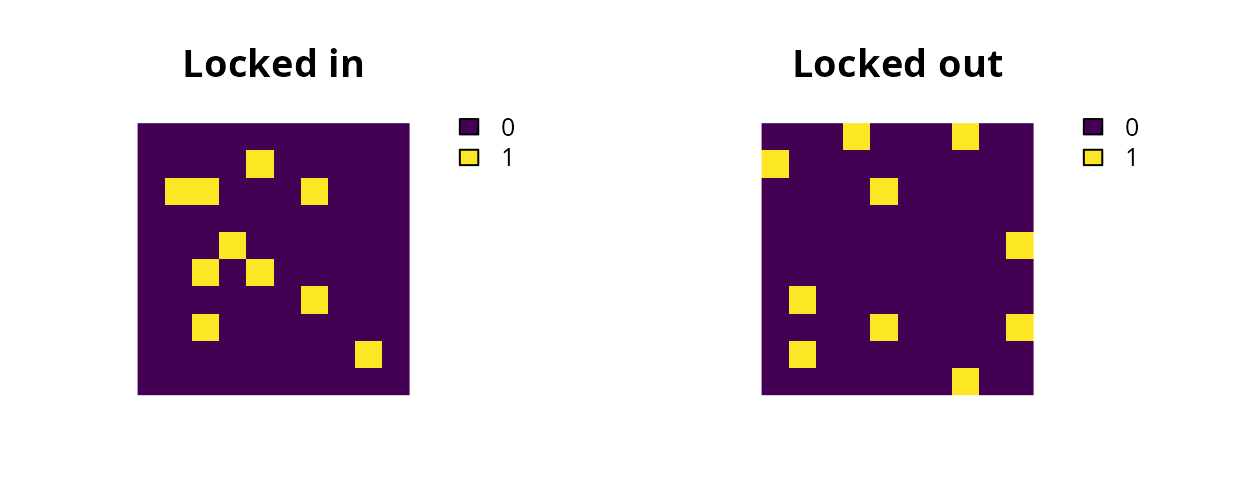
In particular, The add_locked_in_constraints and
add_locked_out_constraints functions are incredibly useful
for real-world conservation planning exercises, so it’s worth pointing
out that there are several ways we can specify which planning units
should be locked in or out of the solutions. If we use raster planning
unit data, we can also use raster data to specify which planning units
should be locked in or locked out.
# load data to lock in or lock out planning units
sim_locked_in_raster <- get_sim_locked_in_raster()
sim_locked_out_raster <- get_sim_locked_out_raster()

# plot the locked data
plot(
  c(sim_locked_in_raster, sim_locked_out_raster),
  xlim = c(-0.1, 1.1), ylim = c(-0.1, 1.1),
  axes = FALSE, main = c("Locked in", "Locked out")
)
# create a problem using raster planning unit data and use the locked raster
# data to lock in some planning units and lock out some other planning units
p25 <-
  problem(sim_pu_raster, sim_features) %>%
  add_min_set_objective() %>%
  add_relative_targets(0.1) %>%
  add_locked_in_constraints(sim_locked_in_raster) %>%
  add_locked_out_constraints(sim_locked_out_raster)

# print problem
print(p25)
## A conservation problem (<ConservationProblem>)
## ├•data
## │├•features: "feature_1", "feature_2", "feature_3", … (5 total)
## │└•planning units:
## │ ├•data: <SpatRaster> (90 total)
## │ ├•costs: continuous values (between 190.1328 and 215.8638)
## │ ├•extent: 0, 0, 1, 1 (xmin, ymin, xmax, ymax)
## │ └•CRS: WGS 84 / Pseudo-Mercator (projected)
## ├•formulation
## │├•objective: minimum set objective
## │├•penalties: none specified
## │├•features:
## ││├•targets: relative targets (all equal to 0.1)
## ││└•weights: none specified
## │├•constraints:
## ││├•1: locked in constraints (10 planning units)
## ││└•2: locked out constraints (10 planning units)
## │└•decisions: binary decision
## └•optimization
## ├•portfolio: single portfolio
## └•solver: gurobi solver (`gap` = 0.1, `time_limit` = 2147483647, …)
## # ℹ Use `summary(...)` to see further details.If our planning unit data are in a spatial vector format (similar to
the sim_pu_polygons data) or a tabular format (similar to
pu_dat), we can use the field names in the data to refer to
which planning units should be locked in and / or out. For example, the
sim_pu_polygons object has TRUE /
FALSE values in the “locked_in” field which indicate which
planning units should be selected in the solution. We could use the data
in this field to specify that those planning units with
TRUE values should be locked in using the following
methods.
# preview sim_pu_polygons object
print(sim_pu_polygons)
## Simple feature collection with 90 features and 3 fields
## Geometry type: POLYGON
## Dimension: XY
## Bounding box: xmin: 0 ymin: 0 xmax: 1 ymax: 1
## Projected CRS: WGS 84 / Pseudo-Mercator
## # A tibble: 90 × 4
## cost locked_in locked_out geom
## * <dbl> <lgl> <lgl> <POLYGON [m]>
## 1 216. FALSE FALSE ((0 1, 0.1 1, 0.1 0.9, 0 0.9, 0 1))
## 2 213. FALSE FALSE ((0.1 1, 0.2 1, 0.2 0.9, 0.1 0.9, 0.1 1))
## 3 207. FALSE FALSE ((0.2 1, 0.3 1, 0.3 0.9, 0.2 0.9, 0.2 1))
## 4 209. FALSE TRUE ((0.3 1, 0.4 1, 0.4 0.9, 0.3 0.9, 0.3 1))
## 5 214. FALSE FALSE ((0.4 1, 0.5 1, 0.5 0.9, 0.4 0.9, 0.4 1))
## 6 214. FALSE FALSE ((0.5 1, 0.6 1, 0.6 0.9, 0.5 0.9, 0.5 1))
## 7 210. FALSE FALSE ((0.6 1, 0.7 1, 0.7 0.9, 0.6 0.9, 0.6 1))
## 8 211. FALSE TRUE ((0.7 1, 0.8 1, 0.8 0.9, 0.7 0.9, 0.7 1))
## 9 210. FALSE FALSE ((0.8 1, 0.9 1, 0.9 0.9, 0.8 0.9, 0.8 1))
## 10 204. FALSE FALSE ((0.9 1, 1 1, 1 0.9, 0.9 0.9, 0.9 1))
## # ℹ 80 more rows
# specify locked in data using the field name
p26 <-
  problem(sim_pu_polygons, sim_features, cost_column = "cost") %>%
  add_min_set_objective() %>%
  add_relative_targets(0.1) %>%
  add_locked_in_constraints("locked_in")

# print problem
print(p26)
## A conservation problem (<ConservationProblem>)
## ├•data
## │├•features: "feature_1", "feature_2", "feature_3", … (5 total)
## │└•planning units:
## │ ├•data: <sf> (90 total)
## │ ├•costs: continuous values (between 190.1328 and 215.8638)
## │ ├•extent: 0, 0, 1, 1 (xmin, ymin, xmax, ymax)
## │ └•CRS: WGS 84 / Pseudo-Mercator (projected)
## ├•formulation
## │├•objective: minimum set objective
## │├•penalties: none specified
## │├•features:
## ││├•targets: relative targets (all equal to 0.1)
## ││└•weights: none specified
## │├•constraints:
## ││└•1: locked in constraints (10 planning units)
## │└•decisions: binary decision
## └•optimization
## ├•portfolio: single portfolio
## └•solver: gurobi solver (`gap` = 0.1, `time_limit` = 2147483647, …)
## # ℹ Use `summary(...)` to see further details.
# specify locked in data using the values in the field
p27 <-
  problem(sim_pu_polygons, sim_features, cost_column = "cost") %>%
  add_min_set_objective() %>%
  add_relative_targets(0.1) %>%
  add_locked_in_constraints(which(sim_pu_polygons$locked_in))

# print problem
print(p27)
## A conservation problem (<ConservationProblem>)
## ├•data
## │├•features: "feature_1", "feature_2", "feature_3", … (5 total)
## │└•planning units:
## │ ├•data: <sf> (90 total)
## │ ├•costs: continuous values (between 190.1328 and 215.8638)
## │ ├•extent: 0, 0, 1, 1 (xmin, ymin, xmax, ymax)
## │ └•CRS: WGS 84 / Pseudo-Mercator (projected)
## ├•formulation
## │├•objective: minimum set objective
## │├•penalties: none specified
## │├•features:
## ││├•targets: relative targets (all equal to 0.1)
## ││└•weights: none specified
## │├•constraints:
## ││└•1: locked in constraints (10 planning units)
## │└•decisions: binary decision
## └•optimization
## ├•portfolio: single portfolio
## └•solver: gurobi solver (`gap` = 0.1, `time_limit` = 2147483647, …)
## # ℹ Use `summary(...)` to see further details.Add penalties
We can also add penalties to a problem to favor or penalize solutions
according to a secondary objective. Unlike the constraint functions,
these functions will add extra information to the objective function of
the optimization function to penalize solutions that do not exhibit
specific characteristics. For example, penalties can be added to a
problem to avoid highly fragmented solutions at the expense of accepting
slightly more expensive solutions. All penalty functions have a
penalty argument that controls the relative importance of
the secondary penalty function compared to the primary objective
function. It is worth noting that incredibly low or incredibly high
penalty values – relative to the main objective function –
can cause problems to take a very long time to solve, so when trying out
a range of different penalty values it can be helpful to limit the
solver to run for a set period of time. The following penalties are
available.
- Boundary penalties: Add penalties to penalize solutions that are excessively fragmented. These penalties are similar to those used in Marxan (Ball et al. 2009; Beyer et al. 2016).
# create problem with penalties that penalize fragmented solutions with a
# penalty factor of 0.01
p28 <-
  problem(sim_pu_raster, sim_features) %>%
  add_min_set_objective() %>%
  add_relative_targets(0.1) %>%
  add_boundary_penalties(penalty = 0.01)

# print problem
print(p28)
## A conservation problem (<ConservationProblem>)
## ├•data
## │├•features: "feature_1", "feature_2", "feature_3", … (5 total)
## │└•planning units:
## │ ├•data: <SpatRaster> (90 total)
## │ ├•costs: continuous values (between 190.1328 and 215.8638)
## │ ├•extent: 0, 0, 1, 1 (xmin, ymin, xmax, ymax)
## │ └•CRS: WGS 84 / Pseudo-Mercator (projected)
## ├•formulation
## │├•objective: minimum set objective
## │├•penalties:
## ││└•1: boundary penalties (`penalty` = 0.01, `edge_factor` = 0.5, …)
## │├•features:
## ││├•targets: relative targets (all equal to 0.1)
## ││└•weights: none specified
## │├•constraints: none specified
## │└•decisions: binary decision
## └•optimization
## ├•portfolio: single portfolio
## └•solver: gurobi solver (`gap` = 0.1, `time_limit` = 2147483647, …)
## # ℹ Use `summary(...)` to see further details.- Neighbor penalties: Add penalties to favor solutions that contain a high number of neighboring planning units (based on Williams et al. 2005). This function is a simpler version of the boundary penalties that may solve faster for large-scale problems.
# create problem with neighbor penalties
p29 <-
  problem(sim_pu_raster, sim_features[[1:4]]) %>%
  add_min_set_objective() %>%
  add_relative_targets(0.1) %>%
  add_neighbor_penalties(penalty = 5)

# print problem
print(p29)
## A conservation problem (<ConservationProblem>)
## ├•data
## │├•features: "feature_1", "feature_2", "feature_3", … (4 total)
## │└•planning units:
## │ ├•data: <SpatRaster> (90 total)
## │ ├•costs: continuous values (between 190.1328 and 215.8638)
## │ ├•extent: 0, 0, 1, 1 (xmin, ymin, xmax, ymax)
## │ └•CRS: WGS 84 / Pseudo-Mercator (projected)
## ├•formulation
## │├•objective: minimum set objective
## │├•penalties:
## ││└•1: neighbor penalties (`penalty` = 5, …)
## │├•features:
## ││├•targets: relative targets (all equal to 0.1)
## ││└•weights: none specified
## │├•constraints: none specified
## │└•decisions: binary decision
## └•optimization
## ├•portfolio: single portfolio
## └•solver: gurobi solver (`gap` = 0.1, `time_limit` = 2147483647, …)
## # ℹ Use `summary(...)` to see further details.- Connectivity penalties: Add penalties to favor solutions that select combinations of planning units with high connectivity between them. This function is used for symmetric connectivities among planning units (based on Önal & Briers 2002).
# create problem with penalties for symmetric connectivity,
# here we will use only the first four layers in
# sim_features for the features and we will use the fifth layer in sim_features
# to represent the connectivity data, where the connectivity_matrix function
# will create a matrix showing the average strength of connectivity between
# adjacent planning units using the data in the fifth layer of sim_features
p30 <-
  problem(sim_pu_raster, sim_features[[1:4]]) %>%
  add_min_set_objective() %>%
  add_relative_targets(0.1) %>%
  add_connectivity_penalties(
    penalty = 5,
    data = connectivity_matrix(sim_pu_raster, sim_features[[5]])
  )

# print problem
print(p30)
## A conservation problem (<ConservationProblem>)
## ├•data
## │├•features: "feature_1", "feature_2", "feature_3", … (4 total)
## │└•planning units:
## │ ├•data: <SpatRaster> (90 total)
## │ ├•costs: continuous values (between 190.1328 and 215.8638)
## │ ├•extent: 0, 0, 1, 1 (xmin, ymin, xmax, ymax)
## │ └•CRS: WGS 84 / Pseudo-Mercator (projected)
## ├•formulation
## │├•objective: minimum set objective
## │├•penalties:
## ││└•1: connectivity penalties (`penalty` = 5, …)
## │├•features:
## ││├•targets: relative targets (all equal to 0.1)
## ││└•weights: none specified
## │├•constraints: none specified
## │└•decisions: binary decision
## └•optimization
## ├•portfolio: single portfolio
## └•solver: gurobi solver (`gap` = 0.1, `time_limit` = 2147483647, …)
## # ℹ Use `summary(...)` to see further details.- Asymmetric connectivity penalties: Add penalties to penalize solutions that select planning units that share high connectivity values with other planning units that are not selected by the solution. This function is used for asymmetric connectivities among planning units (based on Beger et al. 2010).
# create a matrix containing asymmetric connectivity data,
asym_con_matrix <- matrix(
  runif(ncell(sim_pu_raster)^2),
  nrow = ncell(sim_pu_raster),
  ncol = ncell(sim_pu_raster)
)

# create problem with penalties for asymmetric connectivity
p31 <-
  problem(sim_pu_raster, sim_features[[1:4]]) %>%
  add_min_set_objective() %>%
  add_relative_targets(0.1) %>%
  add_asym_connectivity_penalties(penalty = 5, data = asym_con_matrix)

# print problem
print(p31)
## A conservation problem (<ConservationProblem>)
## ├•data
## │├•features: "feature_1", "feature_2", "feature_3", … (4 total)
## │└•planning units:
## │ ├•data: <SpatRaster> (90 total)
## │ ├•costs: continuous values (between 190.1328 and 215.8638)
## │ ├•extent: 0, 0, 1, 1 (xmin, ymin, xmax, ymax)
## │ └•CRS: WGS 84 / Pseudo-Mercator (projected)
## ├•formulation
## │├•objective: minimum set objective
## │├•penalties:
## ││└•1: asymmetric connectivity penalties (`penalty` = 5, …)
## │├•features:
## ││├•targets: relative targets (all equal to 0.1)
## ││└•weights: none specified
## │├•constraints: none specified
## │└•decisions: binary decision
## └•optimization
## ├•portfolio: single portfolio
## └•solver: gurobi solver (`gap` = 0.1, `time_limit` = 2147483647, …)
## # ℹ Use `summary(...)` to see further details.- Linear penalties: Add penalties to penalize solutions that select planning units according to a certain criteria (e.g., anthropogenic pressure).
# create data for penalizing planning units
pen_raster <- simulate_cost(sim_pu_raster)

# create problem with penalties that penalize solutions that select
# planning units with high values in the pen_raster object,
# here we will use a penalty value of 5 to indicate the trade-off (scaling)
# between the penalty values (in the sim_pu_raster) and the main objective
# (i.e., the cost of the solution)
p32 <-
  problem(sim_pu_raster, sim_features) %>%
  add_min_set_objective() %>%
  add_relative_targets(0.1) %>%
  add_linear_penalties(penalty = 5, data = pen_raster)

# print problem
print(p32)
## A conservation problem (<ConservationProblem>)
## ├•data
## │├•features: "feature_1", "feature_2", "feature_3", … (5 total)
## │└•planning units:
## │ ├•data: <SpatRaster> (90 total)
## │ ├•costs: continuous values (between 190.1328 and 215.8638)
## │ ├•extent: 0, 0, 1, 1 (xmin, ymin, xmax, ymax)
## │ └•CRS: WGS 84 / Pseudo-Mercator (projected)
## ├•formulation
## │├•objective: minimum set objective
## │├•penalties:
## ││└•1: linear penalties (`penalty` = 5, …)
## │├•features:
## ││├•targets: relative targets (all equal to 0.1)
## ││└•weights: none specified
## │├•constraints: none specified
## │└•decisions: binary decision
## └•optimization
## ├•portfolio: single portfolio
## └•solver: gurobi solver (`gap` = 0.1, `time_limit` = 2147483647, …)
## # ℹ Use `summary(...)` to see further details.-
Cost penalties: Add penalties to penalize solutions
that select planning units with high cost values. These penalties are a
specialized version of linear constraints (per
add_linear_penalties()) designed to work with the specified cost data.
# create problem with cost penalties, and here we will use a penalty value
# of 0.01 to indicate the trade-off (scaling)
# between the cost values (in the sim_pu_raster) and the main objective
# (i.e., sum of feature shortfall values)
p33 <-
  problem(sim_pu_raster, sim_features) %>%
  add_min_shortfall_objective(budget = 1800) %>%
  add_cost_penalties(0.01) %>%
  add_relative_targets(0.1)

# print problem
print(p33)
## A conservation problem (<ConservationProblem>)
## ├•data
## │├•features: "feature_1", "feature_2", "feature_3", … (5 total)
## │└•planning units:
## │ ├•data: <SpatRaster> (90 total)
## │ ├•costs: continuous values (between 190.1328 and 215.8638)
## │ ├•extent: 0, 0, 1, 1 (xmin, ymin, xmax, ymax)
## │ └•CRS: WGS 84 / Pseudo-Mercator (projected)
## ├•formulation
## │├•objective: minimum shortfall objective (`budget` = 1800)
## │├•penalties:
## ││└•1: cost penalties (`penalty` = 0.01)
## │├•features:
## ││├•targets: relative targets (all equal to 0.1)
## ││└•weights: none specified
## │├•constraints: none specified
## │└•decisions: binary decision
## └•optimization
## ├•portfolio: single portfolio
## └•solver: gurobi solver (`gap` = 0.1, `time_limit` = 2147483647, …)
## # ℹ Use `summary(...)` to see further details.Add the decision types
Conservation planning problems involve making decisions on how planning units will be managed. These decisions are then associated with management actions (e.g., turning a planning unit into a protected area). The type of decision describes how the action is applied to planning units. For instance, the default decision-type is a binary decision type, meaning that we are either selecting or not selecting planning units for management. The following decision types are available.
- Binary decisions: Add a binary decision to a conservation planning problem. This is the classic decision of either prioritizing or not prioritizing a planning unit. Typically, this decision has the assumed action of buying the planning unit to include in a protected area network. If no decision is added to a problem object, then this decision class will be used by default.
# add binary decisions to a problem
p34 <-
  problem(sim_pu_raster, sim_features) %>%
  add_min_set_objective() %>%
  add_relative_targets(0.1) %>%
  add_binary_decisions()

# print problem
print(p34)
## A conservation problem (<ConservationProblem>)
## ├•data
## │├•features: "feature_1", "feature_2", "feature_3", … (5 total)
## │└•planning units:
## │ ├•data: <SpatRaster> (90 total)
## │ ├•costs: continuous values (between 190.1328 and 215.8638)
## │ ├•extent: 0, 0, 1, 1 (xmin, ymin, xmax, ymax)
## │ └•CRS: WGS 84 / Pseudo-Mercator (projected)
## ├•formulation
## │├•objective: minimum set objective
## │├•penalties: none specified
## │├•features:
## ││├•targets: relative targets (all equal to 0.1)
## ││└•weights: none specified
## │├•constraints: none specified
## │└•decisions: binary decision
## └•optimization
## ├•portfolio: single portfolio
## └•solver: gurobi solver (`gap` = 0.1, `time_limit` = 2147483647, …)
## # ℹ Use `summary(...)` to see further details.- Proportion decisions: Add a proportion decision to a problem. This is a relaxed decision where a part of a planning unit can be prioritized, as opposed to the default of the entire planning unit. Typically, this decision has the assumed action of buying a fraction of a planning unit to include in a protected area network. Generally, problems can be solved much faster with proportion-type decisions than binary-type decisions, so they can be very useful when commercial solvers are not available.
# add proportion decisions to a problem
p35 <-
  problem(sim_pu_raster, sim_features) %>%
  add_min_set_objective() %>%
  add_relative_targets(0.1) %>%
  add_proportion_decisions()

# print problem
print(p35)
## A conservation problem (<ConservationProblem>)
## ├•data
## │├•features: "feature_1", "feature_2", "feature_3", … (5 total)
## │└•planning units:
## │ ├•data: <SpatRaster> (90 total)
## │ ├•costs: continuous values (between 190.1328 and 215.8638)
## │ ├•extent: 0, 0, 1, 1 (xmin, ymin, xmax, ymax)
## │ └•CRS: WGS 84 / Pseudo-Mercator (projected)
## ├•formulation
## │├•objective: minimum set objective
## │├•penalties: none specified
## │├•features:
## ││├•targets: relative targets (all equal to 0.1)
## ││└•weights: none specified
## │├•constraints: none specified
## │└•decisions: proportion decision
## └•optimization
## ├•portfolio: single portfolio
## └•solver: gurobi solver (`gap` = 0.1, `time_limit` = 2147483647, …)
## # ℹ Use `summary(...)` to see further details.- Semi-continuous decisions: Add a semi-continuous decision to a problem. This decision is similar to proportion decisions except that it has an upper bound parameter. By default, the decision can range from prioritizing none (0%) to all (100%) of a planning unit. However, a upper bound can be specified to ensure that at most only a fraction (e.g., 80%) of a planning unit can be purchased. This type of decision may be useful when it is not practical to conserve the entire area indicated by a planning unit.
# add semi-continuous decisions to a problem, where we can only manage at most
# 50 % of the area encompassed by a planning unit
p36 <-
  problem(sim_pu_raster, sim_features) %>%
  add_min_set_objective() %>%
  add_relative_targets(0.1) %>%
  add_semicontinuous_decisions(0.5)

# print problem
print(p36)
## A conservation problem (<ConservationProblem>)
## ├•data
## │├•features: "feature_1", "feature_2", "feature_3", … (5 total)
## │└•planning units:
## │ ├•data: <SpatRaster> (90 total)
## │ ├•costs: continuous values (between 190.1328 and 215.8638)
## │ ├•extent: 0, 0, 1, 1 (xmin, ymin, xmax, ymax)
## │ └•CRS: WGS 84 / Pseudo-Mercator (projected)
## ├•formulation
## │├•objective: minimum set objective
## │├•penalties: none specified
## │├•features:
## ││├•targets: relative targets (all equal to 0.1)
## ││└•weights: none specified
## │├•constraints: none specified
## │└•decisions: semicontinuous decision (`upper_limit` = 0.5)
## └•optimization
## ├•portfolio: single portfolio
## └•solver: gurobi solver (`gap` = 0.1, `time_limit` = 2147483647, …)
## # ℹ Use `summary(...)` to see further details.Add a solver
Next, after specifying the mathematical formulation that underpins your conservation planning problem, you can specify how the problem should be solved. If you do not specify this information, the prioritizr R package will automatically use the best solver currently installed on your system with some reasonable defaults. We strongly recommend installing the Gurobi software suite and the gurobi R package to solve problems, and for more information on this topic please refer to the Gurobi Installation Guide. The following solvers are available.
- Gurobi solver: Gurobi is a state of the art commercial optimization software. It is by far the fastest of the solvers that can be used to solve conservation problems. However, it is not freely available. That said, special licenses are available to academics at no cost.
# create a problem and specify that Gurobi should be used to solve the problem
# and specify an optimality gap of zero to obtain the optimal solution
p37 <-
  problem(sim_pu_raster, sim_features) %>%
  add_min_set_objective() %>%
  add_relative_targets(0.1) %>%
  add_binary_decisions() %>%
  add_gurobi_solver(gap = 0)

# print problem
print(p37)
## A conservation problem (<ConservationProblem>)
## ├•data
## │├•features: "feature_1", "feature_2", "feature_3", … (5 total)
## │└•planning units:
## │ ├•data: <SpatRaster> (90 total)
## │ ├•costs: continuous values (between 190.1328 and 215.8638)
## │ ├•extent: 0, 0, 1, 1 (xmin, ymin, xmax, ymax)
## │ └•CRS: WGS 84 / Pseudo-Mercator (projected)
## ├•formulation
## │├•objective: minimum set objective
## │├•penalties: none specified
## │├•features:
## ││├•targets: relative targets (all equal to 0.1)
## ││└•weights: none specified
## │├•constraints: none specified
## │└•decisions: binary decision
## └•optimization
## ├•portfolio: single portfolio
## └•solver: gurobi solver (`gap` = 0, `time_limit` = 2147483647, …)
## # ℹ Use `summary(...)` to see further details.- IBM CPLEX solver: IBM CPLEX is a commercial optimization software. It is faster than the open source solvers available for generating prioritizations (see below), however, it is not freely available. Similar to the Gurobi software, special licenses are available to academics at no cost.
# create a problem and specify that IBM CPLEX should be used to solve the
# problem and specify an optimality gap of zero to obtain the optimal solution
p38 <-
  problem(sim_pu_raster, sim_features) %>%
  add_min_set_objective() %>%
  add_relative_targets(0.1) %>%
  add_binary_decisions() %>%
  add_cplex_solver(gap = 0)

# print problem
print(p38)
## A conservation problem (<ConservationProblem>)
## ├•data
## │├•features: "feature_1", "feature_2", "feature_3", … (5 total)
## │└•planning units:
## │ ├•data: <SpatRaster> (90 total)
## │ ├•costs: continuous values (between 190.1328 and 215.8638)
## │ ├•extent: 0, 0, 1, 1 (xmin, ymin, xmax, ymax)
## │ └•CRS: WGS 84 / Pseudo-Mercator (projected)
## ├•formulation
## │├•objective: minimum set objective
## │├•penalties: none specified
## │├•features:
## ││├•targets: relative targets (all equal to 0.1)
## ││└•weights: none specified
## │├•constraints: none specified
## │└•decisions: binary decision
## └•optimization
## ├•portfolio: single portfolio
## └•solver: cplex solver (`gap` = 0, `time_limit` = 2147483647, …)
## # ℹ Use `summary(...)` to see further details.-
CBC solver: CBC is an open-source
mixed integer programming solver that is part of the Computational
Infrastructure for Operations Research (COIN-OR) project. This solver
seems to have much better performance than the other open-source solvers
(i.e.,
add_rsymphony_solver(),add_lpsymphony_solver()) (see the Solver benchmarks vignette for details). As such, it is strongly recommended to use this solver if the Gurobi and IBM CPLEX solvers are not available. This solver requires the rcbc R package, which is currently only available on GitHub.
# create a problem and specify that CBC should be used to solve the
# problem and specify an optimality gap of zero to obtain the optimal solution
p39 <-
  problem(sim_pu_raster, sim_features) %>%
  add_min_set_objective() %>%
  add_relative_targets(0.1) %>%
  add_binary_decisions() %>%
  add_cbc_solver(gap = 0)

# print problem
print(p39)
## A conservation problem (<ConservationProblem>)
## ├•data
## │├•features: "feature_1", "feature_2", "feature_3", … (5 total)
## │└•planning units:
## │ ├•data: <SpatRaster> (90 total)
## │ ├•costs: continuous values (between 190.1328 and 215.8638)
## │ ├•extent: 0, 0, 1, 1 (xmin, ymin, xmax, ymax)
## │ └•CRS: WGS 84 / Pseudo-Mercator (projected)
## ├•formulation
## │├•objective: minimum set objective
## │├•penalties: none specified
## │├•features:
## ││├•targets: relative targets (all equal to 0.1)
## ││└•weights: none specified
## │├•constraints: none specified
## │└•decisions: binary decision
## └•optimization
## ├•portfolio: single portfolio
## └•solver: cbc solver (`gap` = 0, `time_limit` = 2147483647, …)
## # ℹ Use `summary(...)` to see further details.-
HiGHS solver: HiGHS is an open source
optimization software. Although this solver can have comparable
performance to the CBC solver (i.e.,
add_cbc_solver()) for particular problems and is generally faster than the SYMPHONY based solvers (i.e.,add_rsymphony_solver(),add_lpsymphony_solver()), it can sometimes take much longer than the CBC solver for particular problems. This solver is recommended if theadd_gurobi_solver(),add_cplex_solver(),add_cbc_solver()cannot be used.
# create a problem and specify that HiGHS should be used to solve the
# problem and specify an optimality gap of zero to obtain the optimal solution
p40 <-
  problem(sim_pu_raster, sim_features) %>%
  add_min_set_objective() %>%
  add_relative_targets(0.1) %>%
  add_binary_decisions() %>%
  add_highs_solver(gap = 0)

# print problem
print(p40)
## A conservation problem (<ConservationProblem>)
## ├•data
## │├•features: "feature_1", "feature_2", "feature_3", … (5 total)
## │└•planning units:
## │ ├•data: <SpatRaster> (90 total)
## │ ├•costs: continuous values (between 190.1328 and 215.8638)
## │ ├•extent: 0, 0, 1, 1 (xmin, ymin, xmax, ymax)
## │ └•CRS: WGS 84 / Pseudo-Mercator (projected)
## ├•formulation
## │├•objective: minimum set objective
## │├•penalties: none specified
## │├•features:
## ││├•targets: relative targets (all equal to 0.1)
## ││└•weights: none specified
## │├•constraints: none specified
## │└•decisions: binary decision
## └•optimization
## ├•portfolio: single portfolio
## └•solver: highs solver (`gap` = 0, `time_limit` = 2147483647, …)
## # ℹ Use `summary(...)` to see further details.- lpsymphony solver: SYMPHONY is an open-source integer programming solver that is also part of the COIN-OR project. This solver uses the lpsymphony R package (available on Bioconductor) to interface with the SYMPHONY software.
# create a problem and specify that lpsymphony should be used to solve the
# problem and specify an optimality gap of zero to obtain the optimal solution
p41 <-
  problem(sim_pu_raster, sim_features) %>%
  add_min_set_objective() %>%
  add_relative_targets(0.1) %>%
  add_binary_decisions() %>%
  add_lpsymphony_solver(gap = 0)

# print problem
print(p41)
## A conservation problem (<ConservationProblem>)
## ├•data
## │├•features: "feature_1", "feature_2", "feature_3", … (5 total)
## │└•planning units:
## │ ├•data: <SpatRaster> (90 total)
## │ ├•costs: continuous values (between 190.1328 and 215.8638)
## │ ├•extent: 0, 0, 1, 1 (xmin, ymin, xmax, ymax)
## │ └•CRS: WGS 84 / Pseudo-Mercator (projected)
## ├•formulation
## │├•objective: minimum set objective
## │├•penalties: none specified
## │├•features:
## ││├•targets: relative targets (all equal to 0.1)
## ││└•weights: none specified
## │├•constraints: none specified
## │└•decisions: binary decision
## └•optimization
## ├•portfolio: single portfolio
## └•solver: lpsymphony (`gap` = 0, `time_limit` = 2147483647, …)
## # ℹ Use `summary(...)` to see further details.- Rsymphony solver: This solver provides a different interface to the SYMPHONY software. It uses the Rsymphony R package which is available on The Comprehensive R Archive Network (CRAN). This solver is generally slower than the other solvers, because it cannot use parallel processing.
# create a problem and specify that Rsymphony should be used to solve the
# problem and specify an optimality gap of zero to obtain the optimal solution
p42 <-
  problem(sim_pu_raster, sim_features) %>%
  add_min_set_objective() %>%
  add_relative_targets(0.1) %>%
  add_binary_decisions() %>%
  add_rsymphony_solver(gap = 0)

# print problem
print(p42)
## A conservation problem (<ConservationProblem>)
## ├•data
## │├•features: "feature_1", "feature_2", "feature_3", … (5 total)
## │└•planning units:
## │ ├•data: <SpatRaster> (90 total)
## │ ├•costs: continuous values (between 190.1328 and 215.8638)
## │ ├•extent: 0, 0, 1, 1 (xmin, ymin, xmax, ymax)
## │ └•CRS: WGS 84 / Pseudo-Mercator (projected)
## ├•formulation
## │├•objective: minimum set objective
## │├•penalties: none specified
## │├•features:
## ││├•targets: relative targets (all equal to 0.1)
## ││└•weights: none specified
## │├•constraints: none specified
## │└•decisions: binary decision
## └•optimization
## ├•portfolio: single portfolio
## └•solver: rsymphony solver (`gap` = 0, `time_limit` = 2147483647, …)
## # ℹ Use `summary(...)` to see further details.Add a portfolio
Many conservation planning exercises require a portfolio of solutions. For example, real-world exercises can involve presenting decision makers with a range of near-optimal decisions. Additionally, the number of times that different planning units are selected in different solutions can provide insight into their relative importance. The following portfolio methods are available.
- Gap portfolio: Generate a portfolio of solutions by finding a certain number of solutions that are all within a pre-specified optimality gap. This method is especially useful for generating multiple solutions that can used be to calculate selection frequencies (similar to Marxan). Note that this method requires that the Gurobi optimization software is used to generate solutions.
# create a problem and specify that a portfolio should be created by
# finding five solutions within 10% of optimality
p43 <-
  problem(sim_pu_raster, sim_features) %>%
  add_min_set_objective() %>%
  add_relative_targets(0.1) %>%
  add_binary_decisions() %>%
  add_gap_portfolio(number_solutions = 5, pool_gap = 0.2)

# print problem
print(p43)
## A conservation problem (<ConservationProblem>)
## ├•data
## │├•features: "feature_1", "feature_2", "feature_3", … (5 total)
## │└•planning units:
## │ ├•data: <SpatRaster> (90 total)
## │ ├•costs: continuous values (between 190.1328 and 215.8638)
## │ ├•extent: 0, 0, 1, 1 (xmin, ymin, xmax, ymax)
## │ └•CRS: WGS 84 / Pseudo-Mercator (projected)
## ├•formulation
## │├•objective: minimum set objective
## │├•penalties: none specified
## │├•features:
## ││├•targets: relative targets (all equal to 0.1)
## ││└•weights: none specified
## │├•constraints: none specified
## │└•decisions: binary decision
## └•optimization
## ├•portfolio: gap portfolio (`number_solutions` = 5, `pool_gap` = 0.2)
## └•solver: gurobi solver (`gap` = 0.1, `time_limit` = 2147483647, …)
## # ℹ Use `summary(...)` to see further details.- Top portfolio: Generate a portfolio of solutions by finding a pre-specified number of solutions that are closest to optimality (i.e the top solutions). Note that this method requires that the Gurobi optimization software is used to generate solutions.
# create a problem and specify that a portfolio should be created using
# the top five solutions
p44 <-
  problem(sim_pu_raster, sim_features) %>%
  add_min_set_objective() %>%
  add_relative_targets(0.1) %>%
  add_binary_decisions() %>%
  add_top_portfolio(number_solutions = 5)

# print problem
print(p44)
## A conservation problem (<ConservationProblem>)
## ├•data
## │├•features: "feature_1", "feature_2", "feature_3", … (5 total)
## │└•planning units:
## │ ├•data: <SpatRaster> (90 total)
## │ ├•costs: continuous values (between 190.1328 and 215.8638)
## │ ├•extent: 0, 0, 1, 1 (xmin, ymin, xmax, ymax)
## │ └•CRS: WGS 84 / Pseudo-Mercator (projected)
## ├•formulation
## │├•objective: minimum set objective
## │├•penalties: none specified
## │├•features:
## ││├•targets: relative targets (all equal to 0.1)
## ││└•weights: none specified
## │├•constraints: none specified
## │└•decisions: binary decision
## └•optimization
## ├•portfolio: top portfolio (`number_solutions` = 5)
## └•solver: gurobi solver (`gap` = 0.1, `time_limit` = 2147483647, …)
## # ℹ Use `summary(...)` to see further details.- Extra portfolio: Generate a portfolio of solutions by storing feasible solutions found during the optimization process. Note that this method requires that the Gurobi optimization software is used to generate solutions.
# create a problem and specify that a portfolio should be created using
# extra solutions found while solving the problem
p45 <-
  problem(sim_pu_raster, sim_features) %>%
  add_min_set_objective() %>%
  add_relative_targets(0.1) %>%
  add_binary_decisions() %>%
  add_extra_portfolio()

# print problem
print(p45)
## A conservation problem (<ConservationProblem>)
## ├•data
## │├•features: "feature_1", "feature_2", "feature_3", … (5 total)
## │└•planning units:
## │ ├•data: <SpatRaster> (90 total)
## │ ├•costs: continuous values (between 190.1328 and 215.8638)
## │ ├•extent: 0, 0, 1, 1 (xmin, ymin, xmax, ymax)
## │ └•CRS: WGS 84 / Pseudo-Mercator (projected)
## ├•formulation
## │├•objective: minimum set objective
## │├•penalties: none specified
## │├•features:
## ││├•targets: relative targets (all equal to 0.1)
## ││└•weights: none specified
## │├•constraints: none specified
## │└•decisions: binary decision
## └•optimization
## ├•portfolio: extra portfolio
## └•solver: gurobi solver (`gap` = 0.1, `time_limit` = 2147483647, …)
## # ℹ Use `summary(...)` to see further details.- Cuts portfolio: Generate a portfolio of distinct solutions within a pre-specified optimality gap. This method is only recommended if the Gurobi optimization solver is not available.
# create a problem and specify that a portfolio containing 10 solutions
# should be created using using Bender's cuts
p46 <-
  problem(sim_pu_raster, sim_features) %>%
  add_min_set_objective() %>%
  add_relative_targets(0.1) %>%
  add_binary_decisions() %>%
  add_cuts_portfolio(number_solutions = 10)

# print problem
print(p46)
## A conservation problem (<ConservationProblem>)
## ├•data
## │├•features: "feature_1", "feature_2", "feature_3", … (5 total)
## │└•planning units:
## │ ├•data: <SpatRaster> (90 total)
## │ ├•costs: continuous values (between 190.1328 and 215.8638)
## │ ├•extent: 0, 0, 1, 1 (xmin, ymin, xmax, ymax)
## │ └•CRS: WGS 84 / Pseudo-Mercator (projected)
## ├•formulation
## │├•objective: minimum set objective
## │├•penalties: none specified
## │├•features:
## ││├•targets: relative targets (all equal to 0.1)
## ││└•weights: none specified
## │├•constraints: none specified
## │└•decisions: binary decision
## └•optimization
## ├•portfolio: cuts portfolio (`number_solutions` = 10, `verbose` = TRUE)
## └•solver: gurobi solver (`gap` = 0.1, `time_limit` = 2147483647, …)
## # ℹ Use `summary(...)` to see further details.- Shuffle portfolio: Generate a portfolio of solutions by randomly reordering the data prior to attempting to solve the problem. If the Gurobi optimization solver is not available, this method is the fastest method for generating a set number of solutions within a specified distance from optimality.
# create a problem and specify a portfolio should be created that contains
# 10 solutions and that any duplicate solutions should not be removed
p47 <-
  problem(sim_pu_raster, sim_features) %>%
  add_min_set_objective() %>%
  add_relative_targets(0.1) %>%
  add_binary_decisions() %>%
  add_shuffle_portfolio(number_solutions = 10)

# print problem
print(p47)
## A conservation problem (<ConservationProblem>)
## ├•data
## │├•features: "feature_1", "feature_2", "feature_3", … (5 total)
## │└•planning units:
## │ ├•data: <SpatRaster> (90 total)
## │ ├•costs: continuous values (between 190.1328 and 215.8638)
## │ ├•extent: 0, 0, 1, 1 (xmin, ymin, xmax, ymax)
## │ └•CRS: WGS 84 / Pseudo-Mercator (projected)
## ├•formulation
## │├•objective: minimum set objective
## │├•penalties: none specified
## │├•features:
## ││├•targets: relative targets (all equal to 0.1)
## ││└•weights: none specified
## │├•constraints: none specified
## │└•decisions: binary decision
## └•optimization
## ├•portfolio: shuffle portfolio (`number_solutions` = 10, `threads` = 1, …)
## └•solver: gurobi solver (`gap` = 0.1, `time_limit` = 2147483647, …)
## # ℹ Use `summary(...)` to see further details.Solve the problem
After formulating our conservation planning problem and specifying
how the problem should be solved, we can use the solve()
function to obtain a solution. Note that the solver will typically print
out some information describing the size of the problem and report its
progress when searching for a suitable solution.
# formulate the problem
p48 <-
  problem(sim_pu_raster, sim_features) %>%
  add_min_set_objective() %>%
  add_relative_targets(0.1) %>%
  add_boundary_penalties(penalty = 500, edge_factor = 0.5) %>%
  add_binary_decisions()

# print problem
print(p48)
## A conservation problem (<ConservationProblem>)
## ├•data
## │├•features: "feature_1", "feature_2", "feature_3", … (5 total)
## │└•planning units:
## │ ├•data: <SpatRaster> (90 total)
## │ ├•costs: continuous values (between 190.1328 and 215.8638)
## │ ├•extent: 0, 0, 1, 1 (xmin, ymin, xmax, ymax)
## │ └•CRS: WGS 84 / Pseudo-Mercator (projected)
## ├•formulation
## │├•objective: minimum set objective
## │├•penalties:
## ││└•1: boundary penalties (`penalty` = 500, `edge_factor` = 0.5, …)
## │├•features:
## ││├•targets: relative targets (all equal to 0.1)
## ││└•weights: none specified
## │├•constraints: none specified
## │└•decisions: binary decision
## └•optimization
## ├•portfolio: single portfolio
## └•solver: gurobi solver (`gap` = 0.1, `time_limit` = 2147483647, …)
## # ℹ Use `summary(...)` to see further details.
# solve the problem (using the default solver)
s48 <- solve(p48)
## ## ── Optimization ────────────────────────────────────────────────────────────────## Set parameter Username
## Set parameter LicenseID to value 2806834
## Set parameter TimeLimit to value 2147483647
## Set parameter MIPGap to value 0.1
## Set parameter Presolve to value 2
## Set parameter Threads to value 1
## Academic license - for non-commercial use only - expires 2027-04-14
## Warning: Gurobi version mismatch between R 13.0.1 and C library 13.0.2
## Gurobi Optimizer version 13.0.2 build v13.0.2rc1 (linux64 - "Ubuntu 24.04.2 LTS")
##
## CPU model: 11th Gen Intel(R) Core(TM) i7-1185G7 @ 3.00GHz, instruction set [SSE2|AVX|AVX2|AVX512]
## Thread count: 4 physical cores, 8 logical processors, using up to 1 threads
##
## Non-default parameters:
## TimeLimit 2147483647
## MIPGap 0.1
## Presolve 2
## Threads 1
##
## Optimize a model with 293 rows, 234 columns and 1026 nonzeros (Min)
## Model fingerprint: 0xc085d862
## Model has 234 linear objective coefficients
## Variable types: 144 continuous, 90 integer (90 binary)
## Coefficient statistics:
## Matrix range [2e-01, 1e+00]
## Objective range [2e+02, 7e+02]
## Bounds range [1e+00, 1e+00]
## RHS range [3e+00, 8e+00]
##
## Found heuristic solution: objective 22987.197006
## Found heuristic solution: objective 4212.9617767
## Presolve time: 0.00s
## Presolved: 293 rows, 234 columns, 1026 nonzeros
## Variable types: 0 continuous, 234 integer (234 binary)
## Root relaxation presolved: 293 rows, 234 columns, 1026 nonzeros
##
##
## Root relaxation: objective 2.572718e+03, 199 iterations, 0.00 seconds (0.00 work units)
##
## Nodes | Current Node | Objective Bounds | Work
## Expl Unexpl | Obj Depth IntInf | Incumbent BestBd Gap | It/Node Time
##
## 0 0 2572.71784 0 234 4212.96178 2572.71784 38.9% - 0s
## 0 0 2744.14775 0 196 4212.96178 2744.14775 34.9% - 0s
## H 0 0 3957.3427429 2744.14775 30.7% - 0s
## H 0 0 3894.2509155 2744.14775 29.5% - 0s
## 0 0 2849.78696 0 180 3894.25092 2849.78696 26.8% - 0s
## 0 0 2861.03787 0 185 3894.25092 2861.03787 26.5% - 0s
## 0 0 2861.03787 0 185 3894.25092 2861.03787 26.5% - 0s
## 0 2 2861.21354 0 185 3894.25092 2861.21354 26.5% - 0s
## H 54 50 3724.7123718 2881.34727 22.6% 9.0 0s
## H 54 28 3659.3806915 2881.34727 21.3% 9.0 0s
## H 113 49 3606.4540253 2957.34630 18.0% 14.2 0s
## H 293 87 3548.2596588 3171.74017 10.6% 15.2 0s
##
## Cutting planes:
## Gomory: 3
##
## Explored 304 nodes (5020 simplex iterations) in 0.23 seconds (0.24 work units)
## Thread count was 1 (of 8 available processors)
##
## Solution count 8: 3548.26 3606.45 3659.38 ... 22987.2
##
## Optimal solution found (tolerance 1.00e-01)
## Best objective 3.548259658813e+03, best bound 3.193596607494e+03, gap 9.9954%
# plot solution
plot(
  s48, col = c("grey90", "darkgreen"), main = "Solution",
  xlim = c(-0.1, 1.1), ylim = c(-0.1, 1.1), axes = FALSE
)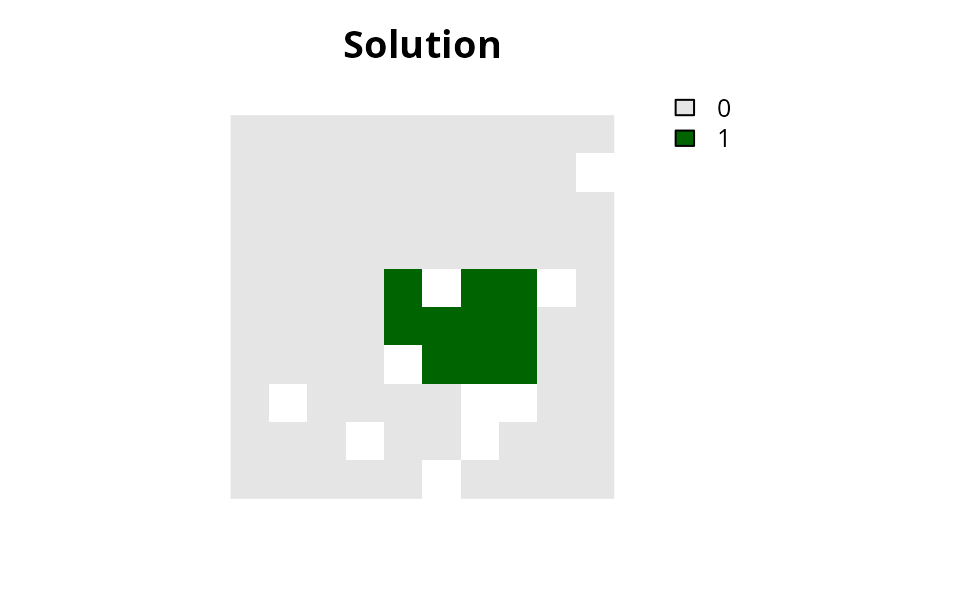
We can plot this solution because the planning unit input data are
spatially referenced in a raster format. The output format will always
match the planning unit data used to initialize the problem. For
example, the solution to a problem with planning units in a spatial
vector (shapefile) format would also be in a spatial vector format.
Similarly, if the planning units were in a tabular format (i.e.,
data.frame), the solution would also be returned in a
tabular format.
We can also extract attributes from the solution that describe the quality of the solution and the optimization process.
# extract the objective value for solution
# (numerical value that is being minimized or maximized during optimization)
print(attr(s48, "objective"))
## solution_1
## 3548.26## solution_1
## 0.248
# extract state message from the solver that describes why this specific
# solution was returned
print(attr(s48, "status"))
## solution_1
## "OPTIMAL"
# extract the objective bound
# (best estimate of lower or upper limit for optimal objective value)
print(attr(s48, "objbound"))
## solution_1
## 0.09995409Evaluate the solution
Conservation planning involves making trade-offs between different criteria (e.g., overall cost, feature representation, connectivity). After obtaining a solution to a conservation planning problem, it is important to evaluate it to help understand the trade-offs made by the prioritization. This is also useful to compare different solutions with each other.
Evaluating performance
Summary statistics can be computed to evaluate the overall performance of a solution based on certain criteria. The following summaries can be computed.
The following functions are available to summarize a solution:
- Number summary: Calculate the number of planning units selected by a solution.
# calculate statistic
eval_n_summary(p48, s48)
## # A tibble: 1 × 2
## summary n
## <chr> <dbl>
## 1 overall 10- Cost summary: Calculate the total cost of a solution.
# calculate statistic
eval_cost_summary(p48, s48)
## # A tibble: 1 × 2
## summary cost
## <chr> <dbl>
## 1 overall 2048.- Feature representation summary: Calculate how well features are represented by a solution. This function can be used for any type of problem.
# calculate statistics
eval_feature_representation_summary(p48, s48)
## # A tibble: 5 × 5
## summary feature total_amount absolute_held relative_held
## <chr> <chr> <dbl> <dbl> <dbl>
## 1 overall feature_1 83.3 8.57 0.103
## 2 overall feature_2 31.2 3.18 0.102
## 3 overall feature_3 72.0 7.28 0.101
## 4 overall feature_4 42.7 5.01 0.118
## 5 overall feature_5 56.7 5.71 0.101- Target coverage summary: Calculate how well representation targets are met by a solution. This function can only be used with problems contain targets.
# calculate statistics
eval_target_coverage_summary(p48, s48)
## # A tibble: 5 × 10
## feature met total_amount absolute_target absolute_held absolute_shortfall
## <chr> <lgl> <dbl> <dbl> <dbl> <dbl>
## 1 feature_1 TRUE 83.3 8.33 8.57 0
## 2 feature_2 TRUE 31.2 3.12 3.18 0
## 3 feature_3 TRUE 72.0 7.20 7.28 0
## 4 feature_4 TRUE 42.7 4.27 5.01 0
## 5 feature_5 TRUE 56.7 5.67 5.71 0
## # ℹ 4 more variables: relative_target <dbl>, relative_held <dbl>,
## # relative_shortfall <dbl>, relative_met <dbl>- Boundary summary: Calculate the total exposed boundary length (perimeter) associated with a solution.
# calculate statistic
eval_boundary_summary(p48, s48)
## # A tibble: 1 × 2
## summary boundary
## <chr> <dbl>
## 1 overall 3- Connectivity summary: Calculate the connectivity of a solution using symmetric connectivity data.
# create symmetric connectivity data
# here we parametrize connectivity based on which planning units are
# adjacent to each other
cm <- adjacency_matrix(sim_pu_raster)

# calculate statistic
eval_connectivity_summary(p48, s48, data = cm)
## # A tibble: 1 × 2
## summary connectivity
## <chr> <dbl>
## 1 overall 24- Asymmetric connectivity summary: Calculate the connectivity of a solution using asymmetric connectivity data.
# create asymmetric connectivity data
# here we parametrize connectivity by randomly simulating values
acm <- matrix(runif(ncell(sim_pu_raster) ^ 2), ncol = ncell(sim_pu_raster))

# calculate statistic
eval_asym_connectivity_summary(p48, s48, data = acm)
## # A tibble: 1 × 2
## summary asym_connectivity
## <chr> <dbl>
## 1 overall 50.1Evaluating importance
Conservation plans can take a long time to implement. Since funding availability and habitat quality can decline over time, it is critical that the most important places in a prioritization are scheduled for management as early as possible. For instance, some planning units in a solution might contain many rare species which do not occur in any other planning units. Alternatively, some planning units might offer an especially high return on investment that reduces costs considerably. As a consequence, conservation planners often need information on which planning units selected in a prioritization are most important to the overall success of the prioritization. To achieve this, conservation planners can use importance scores for each planning unit selected by a solution.
Let’s generate a prioritization so that can compare the different importance methods.
# formulate the problem
p49 <-
  problem(sim_pu_raster, sim_features) %>%
  add_min_set_objective() %>%
  add_relative_targets(0.1) %>%
  add_binary_decisions()

# solve the problem
s49 <- solve(p49)

# plot solution
plot(
  s49, col = c("grey90", "darkgreen"), main = "Solution",
  xlim = c(-0.1, 1.1), ylim = c(-0.1, 1.1), axes = FALSE
)
The following methods are available for computing importance scores.
- Replacement cost: Evaluate importance using the replacement cost method (Cabeza & Moilanen 2006). This method quantifies the importance of a given planning unit as the decrease in the performance of the solution (based on the objective function) if the planning unit cannot be acquired (e.g., in terms of the additional costs required to meet feature targets). The advantages of this method are that it (i) accounts for the costs of the planning units, (ii) can be applied to multiple management zones, (iii) can be applied to any objective function, and (iv) can identify truly irreplaceable planning units (denoted with infinite values). However, the key disadvantage of this method, is that can take an infeasible amount of time to complete for large and complex problems.
# calculate replacement cost scores and make the solver quiet
rc49 <-
  p49 %>%
  add_default_solver(gap = 0, verbose = FALSE) %>%
  eval_replacement_importance(s49)

# plot replacement cost scores
plot(
  rc49, main = "Replacement cost scores",
  xlim = c(-0.1, 1.1), ylim = c(-0.1, 1.1), axes = FALSE
)
- Incremental ranks: Evaluate importance scores by calculating ranks via an incremental optimization process (Jung et al. 2021). Briefly, this approach involves generating incremental prioritizations with increasing budgets, wherein planning units selected in a previous increment are locked in to the following solution. Additionally, locked out constraints are used to ensure that only planning units selected in the original solution are available for selection. The advantages of this approach are that it can (i) be computed relatively quickly for relatively large problems, (ii) account for the cost of different planning units, (iii) account for multiple management zones, and (iv) apply to solutions generated using any objective function.
# calculate rank scores and make the solver quiet
rs49 <-
  p49 %>%
  add_default_solver(gap = 0, verbose = FALSE) %>%
  eval_rank_importance(s49, n = 10)

# plot replacement cost scores
plot(
  rs49, main = "Rank scores",
  xlim = c(-0.1, 1.1), ylim = c(-0.1, 1.1), axes = FALSE
)
- Ferrier method: Evaluate importance by computing irreplaceability scores following Ferrier et al. (2000). The advantages of this method are that it (i) can be computed relatively quickly for moderate problems, and (ii) calculates a score for each feature within each planning unit to provide insight into why certain planning units are more important than others. The disadvantage with this method is that it can only be applied to conservation problems that use targets and have a single zone (i.e., similar to Marxan-type problems).
# calculate Ferrier scores and extract total score
fs49 <- eval_ferrier_importance(p49, s49)[["total"]]

# plot Ferrier scores
plot(
  fs49, main = "Ferrier scores",
  xlim = c(-0.1, 1.1), ylim = c(-0.1, 1.1), axes = FALSE
)
- Rarity weighted richness: Evaluate importance by computing rarity weighted richness scores (Williams et al. 1996). The only advantage with this method is that it can be computed very quickly for very large problems. The key disadvantage with this approach is that it merely describes the spatial patterns of biodiversity, and does not consider any of the goals that underpin conservation planning exercise. For instance, it does not account for planning costs, management zones, objective functions, or feature representation targets.
# calculate rarity weighted richness scores
rwr49 <- eval_rare_richness_importance(p49, s49)

# plot rarity weighted richness scores
plot(
  rwr49, main = "Rarity weighted richness scores",
  xlim = c(-0.1, 1.1), ylim = c(-0.1, 1.1), axes = FALSE
)
In general, we recommend using replacement cost scores for small and moderate sized problems (e.g., less than 30,000 planning units) when it is feasible to do so. It can take a very long time to compute replacement cost scores, and so it is simply not feasible to compute these scores for particularly large problems. For moderate and large sized problems (e.g., more than 30,000 planning units), we recommend using the Ferrier method. This is because it explicitly accounts for representation targets, unlike the rarity weighted richness scores. We almost never recommend using the rarity weighted richness scores. This is because they do not consider criteria needed to inform conservation decision making (Brown et al. 2015).
Multi-objective optimization
Multi-objective optimization provides a framework to examine
trade-offs and identify solutions that represent a desirable compromise
among multiple objectives (López Jaimes et
al. 2011; Neubert et al. 2025). To apply
multi-objective optimization, users should first identify the underlying
motivations and preferences (hereafter, fundamental objectives) that
underpin the planning process and trade-offs they wish to examine (e.g.,
connectivity, representation of different types of features, competing
human uses). For each fundamental objective, users should then formulate
a separate conservation planning problem using the
problem() function. These problem() objects
are then combined into a multi-objective problem with the
multi_problem() function. Next, the
multi_problem() object is customized by adding (i) an
approach to specify a mathematical technique for optimizing multiple
objectives, and (ii) a solver to specify settings for the optimization
software. After completing these steps, the solve()
function is used to generate solutions that aim to achieve multiple
objectives.
When building a multi_problem() object, it is important
to ensure that each problem() object has comparable
planning units, decision types, and zones. For example, if using
terra::rast() planning units, then each
problem() object should have planning units that have the
same resolution, dimensionality (number of rows and columns), and
coordinate reference system. Although the planning units in different
problem() objects can have different values (e.g., one
problem() may have costs based on human pressure and
another problem() may have costs based on spatial area),
they must have missing (NA) values in the same cells (or
rows if planning units are sf::st_sf() objects). If you try
building a multi_problem() object based on
problem() objects that not have comparable planning units,
decision types, and zones, then it will throw an error. Note that each
problem() object can have different planning unit costs,
features, constraints, objectives, and penalties.
Let’s generate a multi-objective conservation problem so that we can compare different approaches. In this example, we have two fundamental objectives: representing keystone species and representing iconic species. Although we ideally want to achieve adequate representation of all species (in other words, meet the representation targets for all species), the total budget available for purchasing planning units is too low to achieve this. As such, we need to generate solutions that weigh these two competing objectives.
# import data
cost_data <- get_sim_pu_raster()
keystone_spp_data <- get_sim_features()[[1:3]]
iconic_spp_data <- get_sim_features()[[4:5]]

# define a total budget (30% of total cost)
budget <- 0.3 * terra::global(cost_data, "sum", na.rm = TRUE)[[1]]

# create problem for keystone fundamental objective
keystone_problem <-
  problem(cost_data, keystone_spp_data) %>%
  add_min_shortfall_objective(budget) %>%
  add_relative_targets(0.4) %>%
  add_binary_decisions()

# print keystone problem
print(keystone_problem)
## A conservation problem (<ConservationProblem>)
## ├•data
## │├•features: "feature_1", "feature_2", and "feature_3" (3 total)
## │└•planning units:
## │ ├•data: <SpatRaster> (90 total)
## │ ├•costs: continuous values (between 190.1328 and 215.8638)
## │ ├•extent: 0, 0, 1, 1 (xmin, ymin, xmax, ymax)
## │ └•CRS: WGS 84 / Pseudo-Mercator (projected)
## ├•formulation
## │├•objective: minimum shortfall objective (`budget` = 5546.159)
## │├•penalties: none specified
## │├•features:
## ││├•targets: relative targets (all equal to 0.4)
## ││└•weights: none specified
## │├•constraints: none specified
## │└•decisions: binary decision
## └•optimization
## ├•portfolio: single portfolio
## └•solver: gurobi solver (`gap` = 0.1, `time_limit` = 2147483647, …)
## # ℹ Use `summary(...)` to see further details.
# create problem for iconic fundamental objective
iconic_problem <-
  problem(cost_data, iconic_spp_data) %>%
  add_min_shortfall_objective(budget) %>%
  add_relative_targets(0.5) %>%
  add_binary_decisions()

# print iconic problem
print(iconic_problem)
## A conservation problem (<ConservationProblem>)
## ├•data
## │├•features: "feature_4" and "feature_5" (2 total)
## │└•planning units:
## │ ├•data: <SpatRaster> (90 total)
## │ ├•costs: continuous values (between 190.1328 and 215.8638)
## │ ├•extent: 0, 0, 1, 1 (xmin, ymin, xmax, ymax)
## │ └•CRS: WGS 84 / Pseudo-Mercator (projected)
## ├•formulation
## │├•objective: minimum shortfall objective (`budget` = 5546.159)
## │├•penalties: none specified
## │├•features:
## ││├•targets: relative targets (all equal to 0.5)
## ││└•weights: none specified
## │├•constraints: none specified
## │└•decisions: binary decision
## └•optimization
## ├•portfolio: single portfolio
## └•solver: gurobi solver (`gap` = 0.1, `time_limit` = 2147483647, …)
## # ℹ Use `summary(...)` to see further details.
# create multi-objective problem
mop <- multi_problem(keystone = keystone_problem, iconic = iconic_problem)

# display multi-objective problem
print(mop)
## A multi-objective conservation problem (<MultiConservationProblem>)
## ├•data
## │└•planning units:
## │ ├•data: <SpatRaster> (90 total)
## │ ├•extent: 0, 0, 1, 1 (xmin, ymin, xmax, ymax)
## │ └•CRS: WGS 84 / Pseudo-Mercator (projected)
## ├•formulation
## │├•name: keystone
## ││├•objective: minimum shortfall objective (`budget` = 5546.159)
## ││├•penalties:
## │││└•1: none specified
## ││└•features: "feature_1", "feature_2", and "feature_3" (3 total)
## ││ ├•targets: relative targets (all equal to 0.4)
## ││ └•weights: none specified
## │├•name: iconic
## ││├•objective: minimum shortfall objective (`budget` = 5546.159)
## ││├•penalties:
## │││└•1: none specified
## ││└•features: "feature_4" and "feature_5" (2 total)
## ││ ├•targets: relative targets (all equal to 0.5)
## ││ └•weights: none specified
## │├•constraints: none specified
## │└•decisions: binary decision
## └•optimization
## ├•approach: none specified
## └•solver: gurobi solver (`gap` = 0.1, `time_limit` = 2147483647, …)
## # ℹ Use `summary(...)` to see further details.-
Weighted sum: This approach linearly combines
multiple objectives using weight (
weights) parameters. In particular, objectives with greater weights are intended to exert greater influence on the optimization process (López Jaimes et al. 2011). Although this approach is conceptually simple and widely used, it is sensitive to differences in scale between objectives (Das & Dennis 1997). Thus the degree of influence that a given objective has on the optimization process may not actually reflect its assigned weight. For example, an objective with a relatively high weight (e.g., 0.99) may have a much smaller influence than an objective with a relatively low weight (e.g., 0.01) if the range of values for the first objective are much smaller than the second objective (e.g., if the objective values for the first objective range between 0 and 1, and the second objective range between 0 and 1000). Due to this limitation, substantial calibration is often required to identify weights that accurately reflect stakeholder preferences and motivations. As such, we generally recommend alternative approaches when possible.
# build multi-objective problem with weighted sum approach and
# specify equal weights for each objective
mop1 <-
  mop %>%
  add_wtd_sum_approach(weights = c(1, 1))

# solve the problem
mos1 <- solve(mop1)

# plot solution
plot(
  mos1, col = c("grey90", "darkgreen"), main = "Solution",
  xlim = c(-0.1, 1.1), ylim = c(-0.1, 1.1), axes = FALSE
)
-
Reference point: This approaches involves combining
the objectives together using (i) reference point
(
ref_points) parameters that specify aspirational levels of achievement for each objective and (ii) weight (weight) parameters that specify the relative importance of each objective (Wierzbicki 1980). It also considers the best (best) and worst (worst) possible objective values for each objective to ensure that differences in scale among objective do not bias the optimization process. To help make this approach accessible, the best and worst objective values are calculated automatically and the reference point values are set based on the best objective values (note, if required, these values can be manually specified). Since setting equal weights for each objective ensures that a solution has (as much as possible) an equal compromise in how close it is to achieving the reference point for each objective, setting weight parameters for this approach is a much more intuitive process than for the weighted sum approach (Deléglise et al. 2024). As such, this approach is especially well-suited for applied contexts that seek to identify solutions that meet multiple stakeholder preferences and motivations (Dujardin & Chadès 2018).
# build multi-objective problem with reference point approach and
# specify equal weights for each objective
mop2 <-
  mop %>%
  add_ref_point_approach(weights = c(1, 1))

# solve the problem
mos2 <- solve(mop2)

# plot solution
plot(
  mos2, col = c("grey90", "darkgreen"), main = "Solution",
  xlim = c(-0.1, 1.1), ylim = c(-0.1, 1.1), axes = FALSE
)
-
Hierarchical: This approach involves solving an
optimization problem for each objective in a hierarchical
(lexicographic) manner. In particular, it solves optimization problems
based on an order of priority, wherein those associated with a higher
priority are solved before those with a lower priority (López Jaimes et al. 2011). By default,
the order of priority is based on the order of problems in the
multi_problem()object. To express trade-offs, this approach uses relative tolerance (rel_tol) parameters that allow the optimization process to degrade previously optimized objectives so that solutions can achieve better performance when optimizing subsequent (lower priority) objectives. This approach is especially well-suited for characterizing the full range of trade-offs between different objectives (in other words, generating a Pareto frontier).
# build multi-objective problem with hierarchical approach and
# specify that the keystone objective should be optimized first
# and performance of the keystone objective can be reduced by 10%
# when subsequently optimizing the iconic objective
mop3 <-
  mop %>%
  add_hier_approach(rel_tol = 0.1)

# solve the problem
mos3 <- solve(mop3)

# plot solution
plot(
  mos3, col = c("grey90", "darkgreen"), main = "Solution",
  xlim = c(-0.1, 1.1), ylim = c(-0.1, 1.1), axes = FALSE
)
The multi-objective optimization approaches can be used to generate
multiple solutions. Although portfolio functions can also be used to
generate multiple solutions, they are different from the approach
functions. This is because the approach functions are designed to
generate solutions that have different levels of performance
(trade-offs) in achieving different objectives, whereas the portfolio
functions are designed to generate solutions that have the
(approximately) same performance with different spatial configurations.
To help explore trade-offs with the approach functions, the
approach_rel_tol_matrix() and
approach_weights_matrix() functions can be used to generate
multiple sets of values for the rel_tol and
weights parameters of approach functions. For example, here
we will use the hierarchical approach and the
approach_rel_tol_matrix() function to generate multiple
solutions and explore trade-offs between representing keystone and
iconic species.
# define a matrix of relative tolerance values between 0 and 1
rel_tol_matrix <-
  approach_rel_tol_matrix(n_problems = 2, n_values = 20, max = 1)

# print matrix
print(rel_tol_matrix)
## [,1]
## [1,] 0.00000000
## [2,] 0.05263158
## [3,] 0.10526316
## [4,] 0.15789474
## [5,] 0.21052632
## [6,] 0.26315789
## [7,] 0.31578947
## [8,] 0.36842105
## [9,] 0.42105263
## [10,] 0.47368421
## [11,] 0.52631579
## [12,] 0.57894737
## [13,] 0.63157895
## [14,] 0.68421053
## [15,] 0.73684211
## [16,] 0.78947368
## [17,] 0.84210526
## [18,] 0.89473684
## [19,] 0.94736842
## [20,] 1.00000000
# build multi-objective problem with hierarchical approach and specify
# gap of 1% to better characterize trade-offs
mop4 <-
  mop %>%
  add_hier_approach(rel_tol = rel_tol_matrix) %>%
  add_default_solver(gap = 0.01)

# generate multiple solutions and remove any duplicates
mos4 <- solve(mop4, remove_duplicates = TRUE)
# plot solutions
plot(
  terra::rast(mos4), col = c("grey90", "darkgreen"),
  xlim = c(-0.1, 1.1), ylim = c(-0.1, 1.1), axes = FALSE
)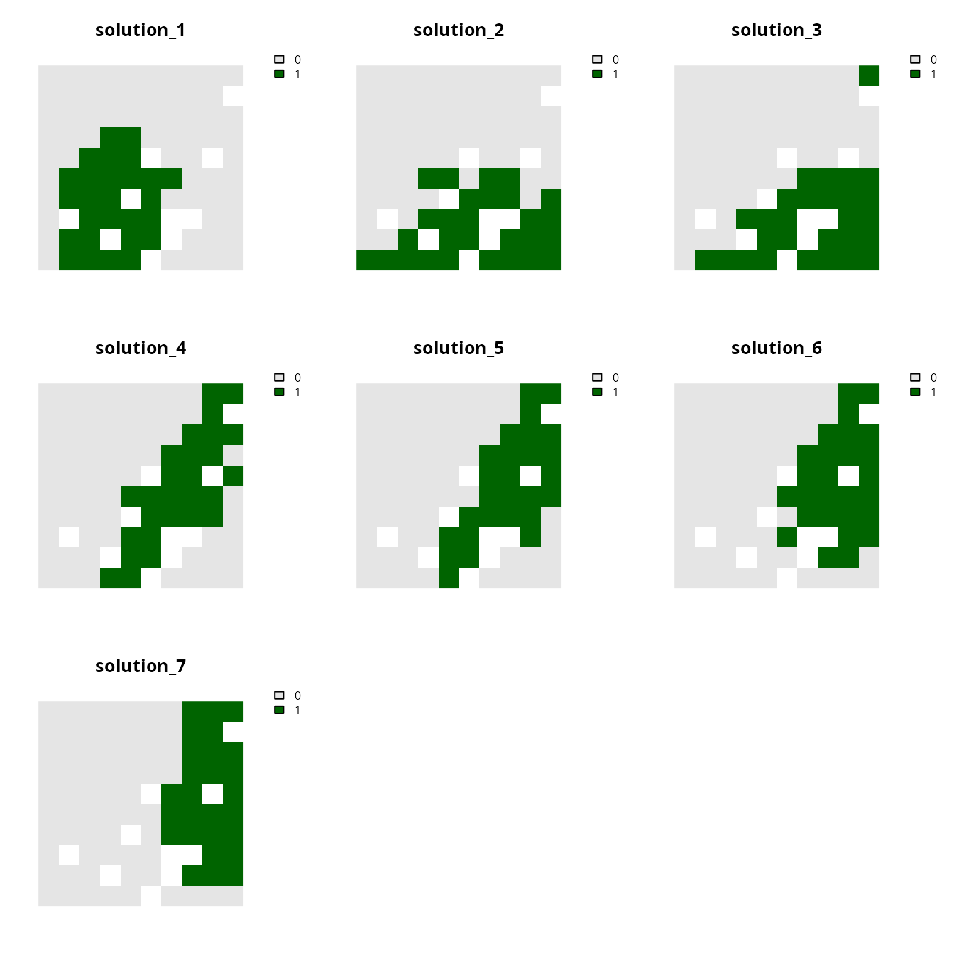
# extract objective values for the solutions
obj_matrix <- attributes(mos4)$objective

# print the objective values
print(obj_matrix)
## keystone iconic
## solution_1 0.8570267 0.9560810
## solution_2 0.9021151 0.8479742
## solution_3 0.9472400 0.8136019
## solution_4 0.9923467 0.7883789
## solution_5 1.0374533 0.7660535
## solution_6 1.0825600 0.7496580
## solution_7 1.1276667 0.7451962
# plot the objectives values to visualize trade-offs
# (note that smaller values are better because these objectives seek to
# minimize representation shortfalls)
plot(
  obj_matrix,
  main = "Trade-offs between objectives",
  xlab = "Keystone objective (shortfall)",
  ylab = "Iconic objective (shortfall)",
  asp = 1
)
Marxan problems
Although we encourage users to build and tailor conservation planning
problems to suit their own needs, sometimes it just simply easier to use
something you’re already familiar with. The
marxan_problem() function is provided as a convenient
wrapper for building and solving Marxan-style conservation
problems. If users already have their conservation planning data
formatted for use with Marxan, this function can also read
Marxan data files and solve the Marxan-style problems
using exact algorithm solvers. Please note that problems built
using the marxan_problem() function are still solved the
same way as a problem initialized using the problem()
function, and therefore still require the installation of one of the
solver packages.
Here is a short example showing how the marxan_problem()
function can be used to read Marxan input files and the
solve function can be used to solve the problem.
# set file path for Marxan input file
minput <- system.file("extdata/marxan/input.dat", package = "prioritizr")

# read Marxan input file
mp <- marxan_problem(minput)

# print problem
print(mp)
## A conservation problem (<ConservationProblem>)
## ├•data
## │├•features: "bird1", "nvis2", "nvis8", "nvis9", … (17 total)
## │└•planning units:
## │ ├•data: <spec_tbl_df> (1751 total)
## │ ├•costs: continuous values (between 0 and 415692.2)
## │ ├•extent: NA
## │ └•CRS: NA
## ├•formulation
## │├•objective: minimum set objective
## │├•penalties:
## ││└•1: boundary penalties (`penalty` = 1, `edge_factor` = 1, …)
## │├•features:
## ││├•targets: relative targets (all equal to 0.3)
## ││└•weights: none specified
## │├•constraints:
## ││├•1: locked in constraints (317 planning units)
## ││└•2: locked out constraints (1 planning units)
## │└•decisions: binary decision
## └•optimization
## ├•portfolio: single portfolio
## └•solver: gurobi solver (`gap` = 0.1, `time_limit` = 2147483647, …)
## # ℹ Use `summary(...)` to see further details.
# solve the problem
ms <- solve(mp)
# since the Marxan data was in a tabular format, the solution is also returned
# in a tabular format, so we will print the first six rows of the table
# containing the solution
head(ms)
## # A tibble: 6 × 8
## id cost status xloc yloc locked_in locked_out solution_1
## <dbl> <dbl> <dbl> <dbl> <dbl> <lgl> <lgl> <dbl>
## 1 3 0 0 1116623. -4493479. FALSE FALSE 0
## 2 30 7527. 3 1110623. -4496943. FALSE TRUE 0
## 3 56 37349. 0 1092623. -4500408. FALSE FALSE 0
## 4 58 16959. 0 1116623. -4500408. FALSE FALSE 0
## 5 84 34220. 0 1098623. -4503872. FALSE FALSE 0
## 6 85 178908. 0 1110623. -4503872. FALSE FALSE 0Alternatively, rather then using a Marxan input file to
construct the problem, we can manually read in the Marxan data
files and input these to the marxan_problem() function.
# load data
pu <-
  system.file("extdata/marxan/input/pu.dat", package = "prioritizr") %>%
  read.table(sep = ",", header = TRUE)
features <-
  system.file("extdata/marxan/input/spec.dat", package = "prioritizr") %>%
  read.table(sep = ",", header = TRUE)
bound <-
  system.file("extdata/marxan/input/bound.dat", package = "prioritizr") %>%
  read.table(sep = "\t", header = TRUE)
rij <-
  system.file("extdata/marxan/input/puvspr.dat", package = "prioritizr") %>%
  read.table(sep = ",", header = TRUE)

# build Marxan problem using data.frame objects
mp2 <- marxan_problem(
  x = pu, spec = features, puvspr = rij, bound = bound, blm = 0
)

# print problem
print(mp2)
## A conservation problem (<ConservationProblem>)
## ├•data
## │├•features: "bird1", "nvis2", "nvis8", "nvis9", … (17 total)
## │└•planning units:
## │ ├•data: <data.frame> (1751 total)
## │ ├•costs: continuous values (between 0 and 415692.2)
## │ ├•extent: NA
## │ └•CRS: NA
## ├•formulation
## │├•objective: minimum set objective
## │├•penalties:
## ││└•1: boundary penalties (`penalty` = 0, `edge_factor` = 1, …)
## │├•features:
## ││├•targets: relative targets (all equal to 0.3)
## ││└•weights: none specified
## │├•constraints:
## ││├•1: locked in constraints (317 planning units)
## ││└•2: locked out constraints (1 planning units)
## │└•decisions: binary decision
## └•optimization
## ├•portfolio: single portfolio
## └•solver: gurobi solver (`gap` = 0.1, `time_limit` = 2147483647, …)
## # ℹ Use `summary(...)` to see further details.Conservation planning problems that are built using the
marxan_problem() function can also be customized. For
example, we could change the decision type for mp2 to
involve selecting a proportion of each planing unit (using the
add_proportion_decisions() function).
Conclusion
Hopefully, this vignette has provided an informative overview of the prioritizr R package. For more examples using the package, please see the other vignettes. Perhaps, one of the best ways to learn a new piece of software is to just try it out. Test it, try breaking it, make mistakes, and learn from them. We would recommend trying to build conservation planning problems that resemble those you face in your own work—but using the built-in example data sets. This way you can quickly verify that the problems you build actually mean what you think they mean. For instance, you can try playing around with the targets and see what effect they have on the solutions, or try playing around with penalties and see what effect they have on the solutions. Finally, if you have any questions about using the package or suggestions for it, please post an issue on the package’s online coding repository.