Generate a portfolio of solutions for a conservation planning problem by storing feasible solutions discovered during the optimization process. This method is useful for quickly obtaining multiple solutions, but does not provide any guarantees on the number of solutions, or the quality of solutions.
Arguments
- x
problem()object.
Value
An updated problem() object with the portfolio added to it.
Details
This strategy for generating a portfolio requires problems to
be solved using the Gurobi software (i.e., using
add_gurobi_solver(). Specifically, version 8.0.0 (or greater)
of the gurobi package must be installed.
See also
Other functions for adding portfolios:
add_cuts_portfolio(),
add_default_portfolio(),
add_gap_portfolio(),
add_shuffle_portfolio(),
add_single_portfolio(),
add_top_portfolio()
Examples
# set seed for reproducibility
set.seed(600)
# load data
sim_pu_raster <- get_sim_pu_raster()
sim_features <- get_sim_features()
sim_zones_pu_raster <- get_sim_zones_pu_raster()
sim_zones_features <- get_sim_zones_features()
# create minimal problem with a portfolio for extra solutions
p1 <-
problem(sim_pu_raster, sim_features) %>%
add_min_set_objective() %>%
add_relative_targets(0.05) %>%
add_extra_portfolio() %>%
add_default_solver(gap = 0, verbose = FALSE)
# solve problem and generate portfolio
s1 <- solve(p1)
# convert portfolio into a multi-layer raster object
s1 <- terra::rast(s1)
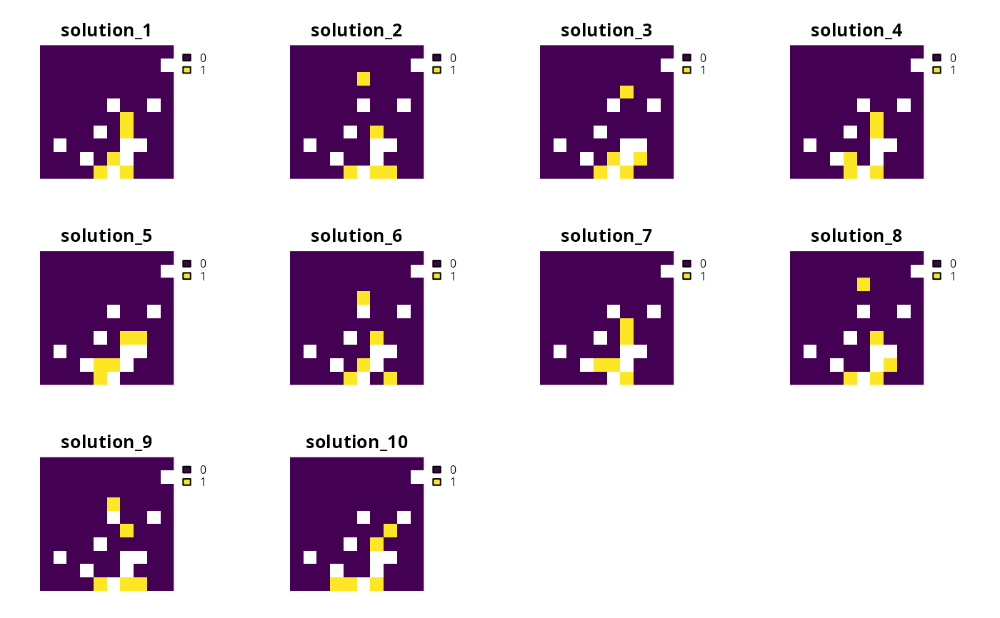
# print number of solutions found
print(terra::nlyr(s1))
#> [1] 10
# plot solutions
plot(s1, axes = FALSE)
 # create multi-zone problem with a portfolio for extra solutions
p2 <-
problem(sim_zones_pu_raster, sim_zones_features) %>%
add_min_set_objective() %>%
add_relative_targets(matrix(runif(15, 0.1, 0.2), nrow = 5, ncol = 3)) %>%
add_extra_portfolio() %>%
add_default_solver(gap = 0, verbose = FALSE)
# solve problem and generate portfolio
s2 <- solve(p2)
# convert each solution in the portfolio into a single category layer
s2 <- terra::rast(lapply(s2, category_layer))
# print number of solutions found
print(terra::nlyr(s2))
#> [1] 10
# plot solutions in portfolio
plot(s2, axes = FALSE)
# create multi-zone problem with a portfolio for extra solutions
p2 <-
problem(sim_zones_pu_raster, sim_zones_features) %>%
add_min_set_objective() %>%
add_relative_targets(matrix(runif(15, 0.1, 0.2), nrow = 5, ncol = 3)) %>%
add_extra_portfolio() %>%
add_default_solver(gap = 0, verbose = FALSE)
# solve problem and generate portfolio
s2 <- solve(p2)
# convert each solution in the portfolio into a single category layer
s2 <- terra::rast(lapply(s2, category_layer))
# print number of solutions found
print(terra::nlyr(s2))
#> [1] 10
# plot solutions in portfolio
plot(s2, axes = FALSE)