Add a Gurobi solver

Specify that the Gurobi software should be used to solve a conservation planning problem (Gurobi Optimization LLC 2021). This function can also be used to customize the behavior of the solver. It requires the gurobi package to be installed (see below for installation instructions).

Usage

add_gurobi_solver(
  x,
  gap = 0.1,
  time_limit = .Machine$integer.max,
  presolve = 2,
  threads = 1,
  first_feasible = FALSE,
  numeric_focus = FALSE,
  node_file_start = Inf,
  start_solution = NULL,
  verbose = TRUE
)

Arguments

x: problem() object.
gap: numeric gap to optimality. This gap is relative and expresses the acceptable deviance from the optimal objective. For example, a value of 0.01 will result in the solver stopping when it has found a solution within 1% of optimality. Additionally, a value of 0 will result in the solver stopping when it has found an optimal solution. The default value is 0.1 (i.e., 10% from optimality).
time_limit: numeric time limit (seconds) for generating solutions. The solver will return the current best solution when this time limit is exceeded. The default value is the largest integer value (i.e., .Machine$integer.max), effectively meaning that solver will keep running until a solution within the optimality gap is found.
presolve: integer number indicating how intensively the solver should try to simplify the problem before solving it. Available options are: (-1) automatically determine the intensity of pre-solving, (0) disable pre-solving, (1) conservative level of pre-solving, and (2) very aggressive level of pre-solving . The default value is 2.
threads: integer number of threads to use for the optimization algorithm. The default value is 1.
first_feasible: logical should the first feasible solution be be returned? If first_feasible is set to TRUE, the solver will return the first solution it encounters that meets all the constraints, regardless of solution quality. Note that the first feasible solution is not an arbitrary solution, rather it is derived from the relaxed solution, and is therefore often reasonably close to optimality. Defaults to FALSE.
numeric_focus: logical should extra attention be paid to verifying the accuracy of numerical calculations? This may be useful when dealing with problems that may suffer from numerical instability issues. Beware that it will likely substantially increase run time (sets the Gurobi NumericFocus parameter to 3). Defaults to FALSE.
node_file_start: numeric threshold amount of memory (in GB). Once the amount of memory (RAM) used to store information for solving the optimization problem exceeds this parameter value, the solver will begin storing this information on disk (using the Gurobi NodeFileStart parameter). This functionality is useful if the system has insufficient memory to solve a given problem (e.g., solving the problem with default settings yields the OUT OF MEMORY error message) and a system with more memory is not readily available. For example, a value of 4 indicates that the solver will start using the disk after it uses more than 4 GB of memory to store information on solving the problem. Defaults to Inf such that the solver will not attempt to store information on disk when solving a given problem.
start_solution: NULL or object containing the starting solution for the solver. This is can be useful because specifying a starting solution can speed up the optimization process. Defaults to NULL such that no starting solution is used. To specify a starting solution, the argument to start_solution should be in the same format as the planning units (i.e., a NULL, numeric, matrix, data.frame, terra::rast(), or sf::sf() object). See the Start solution format section for more information.
verbose: logical should information be printed while solving optimization problems? Defaults to TRUE.

Value

An updated problem() object with the solver added to it.

Details

Gurobi is a state-of-the-art commercial optimization software with an R package interface. It is by far the fastest of the solvers available for generating prioritizations, however, it is not freely available. That said, licenses are available to academics at no cost. The gurobi package is distributed with the Gurobi software suite. This solver uses the gurobi package to solve problems. For information on the performance of different solvers, please see Schuster et al. (2020) for benchmarks comparing the run time and solution quality of different solvers when applied to different sized datasets.

Installation

Please see the Gurobi Installation Guide vignette for details on installing the Gurobi software and the gurobi package. You can access this vignette online or using the following code:

vignette("gurobi_installation_guide", package = "prioritizr")

Start solution format

Broadly speaking, the argument to start_solution must be in the same format as the planning unit data in the argument to x. Further details on the correct format are listed separately for each of the different planning unit data formats:

x has numeric planning units: The argument to start_solution must be a numeric vector with each element corresponding to a different planning unit. It should have the same number of planning units as those in the argument to x. Additionally, any planning units missing cost (NA) values should also have missing (NA) values in the argument to start_solution.
x has matrix planning units: The argument to start_solution must be a matrix vector with each row corresponding to a different planning unit, and each column correspond to a different management zone. It should have the same number of planning units and zones as those in the argument to x. Additionally, any planning units missing cost (NA) values for a particular zone should also have a missing (NA) values in the argument to start_solution.
x has terra::rast() planning units: The argument to start_solution be a terra::rast() object where different grid cells (pixels) correspond to different planning units and layers correspond to a different management zones. It should have the same dimensionality (rows, columns, layers), resolution, extent, and coordinate reference system as the planning units in the argument to x. Additionally, any planning units missing cost (NA) values for a particular zone should also have missing (NA) values in the argument to start_solution.
x has data.frame planning units: The argument to start_solution must be a data.frame with each column corresponding to a different zone, each row corresponding to a different planning unit, and cell values corresponding to the solution value. This means that if a data.frame object containing the solution also contains additional columns, then these columns will need to be subsetted prior to using this function (see below for example with sf::sf() data). Additionally, any planning units missing cost (NA) values for a particular zone should also have missing (NA) values in the argument to start_solution.
x has sf::sf() planning units: The argument to start_solution must be a sf::sf() object with each column corresponding to a different zone, each row corresponding to a different planning unit, and cell values corresponding to the solution value. This means that if the sf::sf() object containing the solution also contains additional columns, then these columns will need to be subsetted prior to using this function (see below for example). Additionally, the argument to start_solution must also have the same coordinate reference system as the planning unit data. Furthermore, any planning units missing cost (NA) values for a particular zone should also have missing (NA) values in the argument to start_solution.

References

Gurobi Optimization LLC (2021) Gurobi Optimizer Reference Manual. https://www.gurobi.com.

Schuster R, Hanson JO, Strimas-Mackey M, and Bennett JR (2020). Exact integer linear programming solvers outperform simulated annealing for solving conservation planning problems. PeerJ, 8: e9258.

Examples

# \dontrun{
# load data
sim_pu_raster <- get_sim_pu_raster()
sim_features <- get_sim_features()

# create problem
p1 <-
  problem(sim_pu_raster, sim_features) %>%
  add_min_set_objective() %>%
  add_relative_targets(0.1) %>%
  add_binary_decisions() %>%
  add_gurobi_solver(gap = 0, verbose = FALSE)

# generate solution
s1 <- solve(p1)

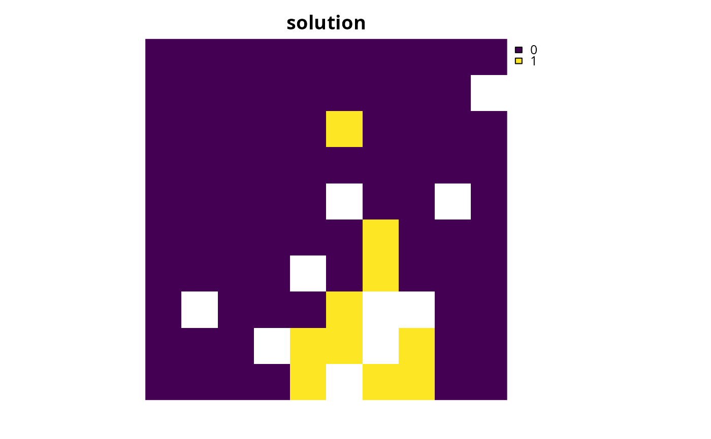
# plot solution
plot(s1, main = "solution", axes = FALSE)


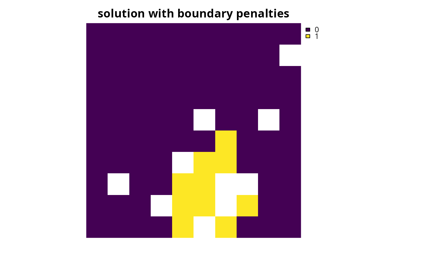
# create a similar problem with boundary length penalties and
# specify the solution from the previous run as a starting solution
p2 <-
  problem(sim_pu_raster, sim_features) %>%
  add_min_set_objective() %>%
  add_relative_targets(0.1) %>%
  add_boundary_penalties(10) %>%
  add_binary_decisions() %>%
  add_gurobi_solver(gap = 0, start_solution = s1, verbose = FALSE)

# generate solution
s2 <- solve(p2)

# plot solution
plot(s2, main = "solution with boundary penalties", axes = FALSE)

# }