Add penalties to a conservation planning problem to favor solutions that spatially clump planning units together based on the overall boundary length (i.e., total perimeter).
Usage
# S4 method for class 'ConservationProblem,ANY,ANY,ANY,ANY,data.frame'
add_boundary_penalties(x, penalty, edge_factor, formulation, zones, data)

# S4 method for class 'ConservationProblem,ANY,ANY,ANY,ANY,matrix'
add_boundary_penalties(x, penalty, edge_factor, formulation, zones, data)

# S4 method for class 'ConservationProblem,ANY,ANY,ANY,ANY,ANY'
add_boundary_penalties(x, penalty, edge_factor, formulation, zones, data)
Arguments
- x
problem()object.- penalty
numericvalue denoting the importance of selecting planning units that are spatially clumped together compared to the main problem objective (e.g., solution cost ifxhas a minimum set objective peradd_min_set_objective()). Higherpenaltyvalues prefer solutions with a higher degree of spatial clumping, and smallerpenaltyvalues prefer solutions with a smaller degree of clumping. Note that negativepenaltyvalues prefer solutions that are spatially fragmented. This parameter is equivalent to the boundary length modifier (BLM) parameter in Marxan.- edge_factor
numericvalue or vector denoting the proportion for scaling planning unit edges (borders) that do not have any neighboring planning units. For example, an edge factor of0.5is commonly used to avoid overly penalizing planning units along coastlines. Note thatedge_factormust have a value for each zone inx.- formulation
charactervalue denoting the name of the linearization technique used to formulate the penalties. Available options are"simple"and"knapsack". Defaults to"simple". If you are having issues with solving problems within a reasonable period of time usingformulation = "simple", then consider tryingformulation = "knapsack". Note that theformulation = "knapsack"is likely to yield better performance when each planning unit has a large number of neighbors (e.g., planning units are based on a hexagonal grid or irregular polygons).- zones
matrixorMatrixobject describing the clumping scheme for different zones. Each row and column corresponds to a different zone inx, and cell values indicate the relative importance of clumping planning units that are allocated to a combination of zones. Cell values along the diagonal of the matrix represent the relative importance of clumping planning units that are allocated to the same zone. Cell values must range between 1 and -1, where negative values favor solutions that spread out planning units. Defaults to an identity matrix (i.e., a matrix with ones along the matrix diagonal and zeros elsewhere), so that penalties are incurred when neighboring planning units are not assigned to the same zone. If the cells along the matrix diagonal contain markedly smaller values than those found elsewhere in the matrix, then solutions are preferred that surround planning units with those allocated to different zones (i.e., greater spatial fragmentation of zones).- data
NULL,data.frame,matrix, orMatrixobject containing the boundary data. These data describe the total amount of boundary (perimeter) length for each planning unit, and the amount of boundary (perimeter) length shared between different planning units (i.e., planning units that are adjacent to each other). See the Data format section for more information.
Value
An updated problem() object with the penalties added to it.
Details
This function adds penalties to a conservation planning problem
to penalize fragmented solutions. It was is inspired by Ball et al.
(2009) and Beyer et al. (2016). Indeed, penalty is
equivalent to the boundary length modifier (BLM) used in
Marxan.
Note that this function can only
be used to represent symmetric relationships between planning units. If
asymmetric relationships are required, use the
add_connectivity_penalties() function.
Data format
The following formats can be used to specify data.
Note that boundary data must always describe symmetric relationships
between planning units.
dataas aNULLvalueHere boundary length data are automatically calculated using the
boundary_matrix()function and then rescaled withrescale_matrix(). This is the default fordata. Note that the boundary data must be supplied using one of the other formats below ifxdoes not contain planning units that are spatially referenced. (e.g., planning unit data are adata.frameobject ornumericvector).dataas amatrix/MatrixobjectHere rows and columns correspond to different planning units and cell values represent the amount of boundary length shared between two planning units. Cells along the matrix diagonal denote the total boundary length associated with each planning unit. For example, boundary data in this format can be generated with the
boundary_matrix()function.dataas adata.frameobjectHere rows correspond to a pair of planning units and columns provide information about each pair of planning units. In particular,
datamust have the columns:"id1","id2", and"boundary". The"id1"and"id2"columns contain identifiers (indices) for a pair of planning units, and the"boundary"column contains the amount of shared boundary length between these two planning units. Additionally, if the"id1"and"id2"columns contain the same values, then the value denotes the amount of exposed boundary length (not total boundary) for that particular planning unit. This format follows the the standard Marxan format for boundary data (i.e., per the "bound.dat" file).
Mathematical formulation
The boundary penalties are implemented using the following equations. Let
\(I\) represent the set of planning units
(indexed by \(i\) or \(j\)), \(Z\) represent
the set of management zones (indexed by \(z\) or \(y\)), and
\(X_{iz}\) represent the decision
variable for planning unit \(i\) for in zone \(z\) (e.g., with binary
values one indicating if planning unit is allocated or not). Also, let
\(p\) represent penalty, \(E_z\) represent edge_factor,
\(B_{ij}\) represent data in matrix format
(e.g., generated using boundary_matrix()), and
\(W_{zz}\) represent zones in matrix format.
$$ \sum_{i}^{I} \sum_{z}^{Z} (p \times W_{zz} B_{ii}) + \sum_{i}^{I} \sum_{j}^{I} \sum_{z}^{Z} \sum_{y}^{Z} (-2 \times p \times X_{iz} \times X_{jy} \times W_{zy} \times B_{ij})$$
Note that when the problem objective is to maximize some measure of benefit and not minimize some measure of cost, the term \(p\) is replaced with \(-p\). Additionally, to linearize the problem, the expression \(X_{iz} \times X_{jy}\) is modeled using a set of continuous variables (bounded between 0 and 1) based on Beyer et al. (2016).
References
Ball IR, Possingham HP, and Watts M (2009) Marxan and relatives: Software for spatial conservation prioritisation in Spatial conservation prioritisation: Quantitative methods and computational tools. Eds Moilanen A, Wilson KA, and Possingham HP. Oxford University Press, Oxford, UK.
Beyer HL, Dujardin Y, Watts ME, and Possingham HP (2016) Solving conservation planning problems with integer linear programming. Ecological Modelling, 228: 14–22.
See also
See penalties for an overview of all functions for adding penalties.
Also see add_neighbor_penalties() for a penalty that
can reduce spatial fragmentation and has faster solver run times.
Additionally, see calibrate_cohon_penalty() for assistance with selecting
an appropriate penalty value.
Other functions for adding penalties:
add_asym_connectivity_penalties(),
add_connectivity_penalties(),
add_cost_penalties(),
add_feature_weights(),
add_linear_penalties(),
add_neighbor_penalties()
Examples
# set seed for reproducibility
set.seed(500)
# load data
sim_pu_raster <- get_sim_pu_raster()
sim_features <- get_sim_features()
sim_zones_pu_raster <- get_sim_zones_pu_raster()
sim_zones_features <- get_sim_zones_features()
# create minimal problem
p1 <-
problem(sim_pu_raster, sim_features) %>%
add_min_set_objective() %>%
add_relative_targets(0.2) %>%
add_binary_decisions() %>%
add_default_solver(verbose = FALSE)
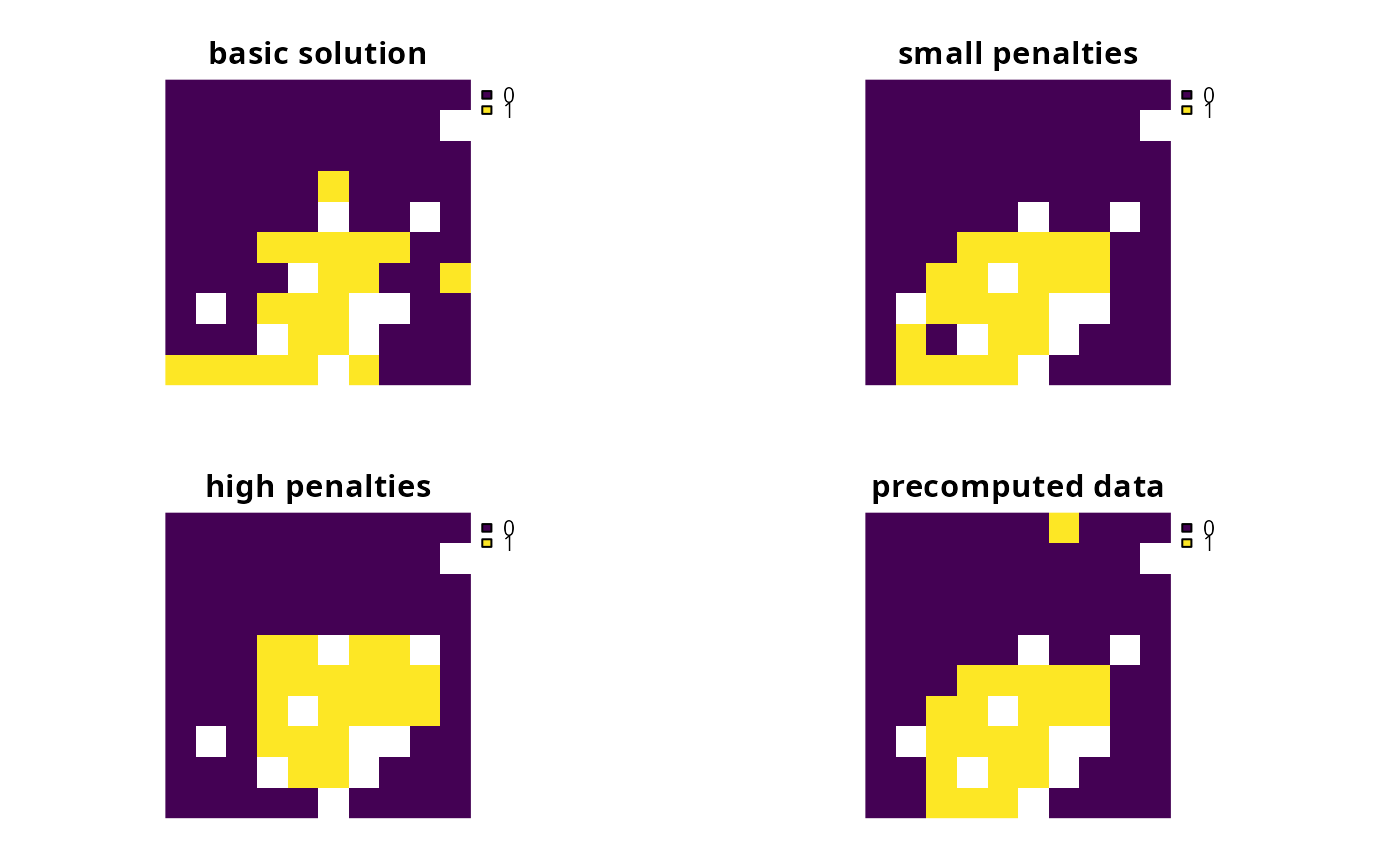
# create problem with low boundary penalties
p2 <- p1 %>% add_boundary_penalties(50, 1)
# create problem with high boundary penalties but outer edges receive
# half the penalty as inner edges
p3 <- p1 %>% add_boundary_penalties(500, 0.5)
# create a problem using precomputed boundary data
bmat <- boundary_matrix(sim_pu_raster)
p4 <- p1 %>% add_boundary_penalties(50, 1, data = bmat)
# solve problems
s1 <- c(solve(p1), solve(p2), solve(p3), solve(p4))
names(s1) <- c("basic solution", "small penalties", "high penalties",
"precomputed data"
)
# plot solutions
plot(s1, axes = FALSE)
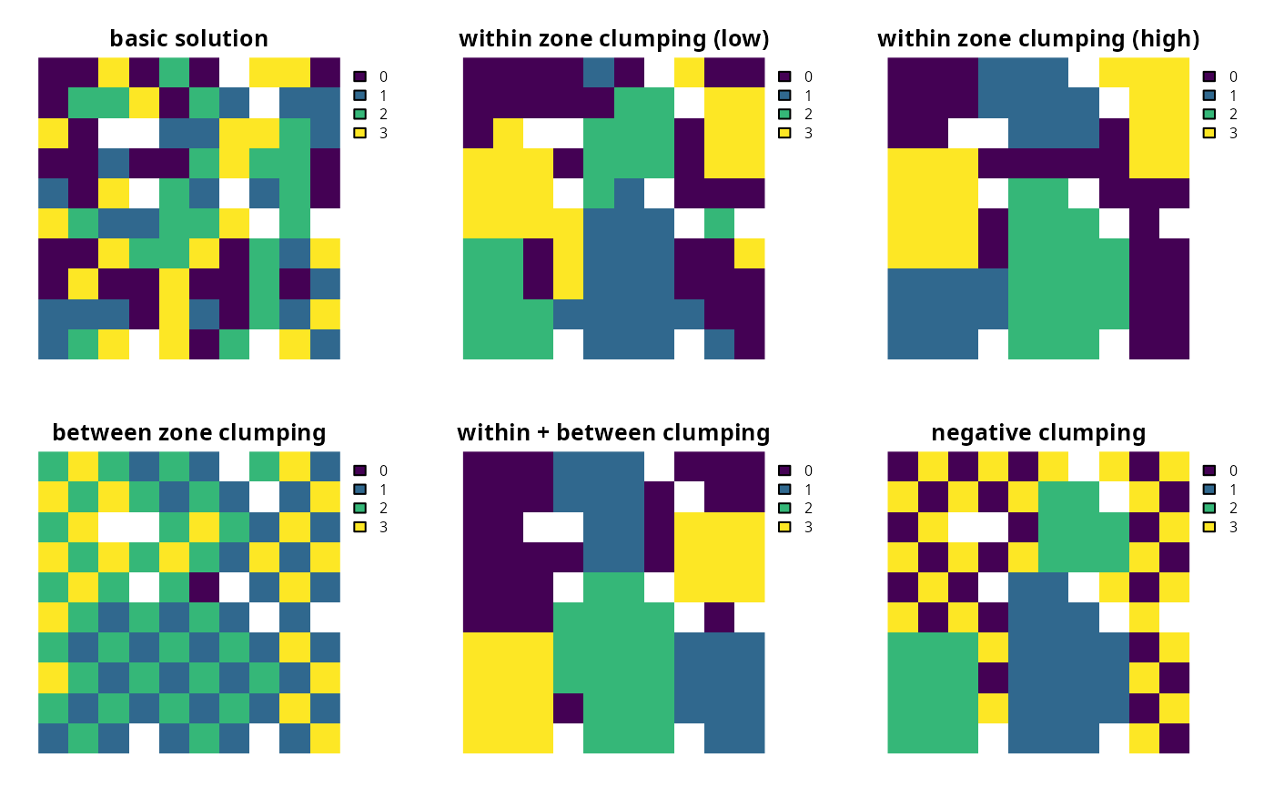
 # create minimal problem with multiple zones and limit the run-time for
# solver to 10 seconds so this example doesn't take too long
p5 <-
problem(sim_zones_pu_raster, sim_zones_features) %>%
add_min_set_objective() %>%
add_relative_targets(matrix(0.2, nrow = 5, ncol = 3)) %>%
add_binary_decisions() %>%
add_default_solver(time_limit = 10, verbose = FALSE)
# create zone matrix which favors clumping planning units that are
# allocated to the same zone together - note that this is the default
zm6 <- diag(3)
print(zm6)
#> [,1] [,2] [,3]
#> [1,] 1 0 0
#> [2,] 0 1 0
#> [3,] 0 0 1
# create problem with the zone matrix and low penalties
p6 <- p5 %>% add_boundary_penalties(50, zone = zm6)
# create another problem with the same zone matrix and higher penalties
p7 <- p5 %>% add_boundary_penalties(500, zone = zm6)
# create zone matrix which favors clumping units that are allocated to
# different zones together
zm8 <- matrix(1, ncol = 3, nrow = 3)
diag(zm8) <- 0
print(zm8)
#> [,1] [,2] [,3]
#> [1,] 0 1 1
#> [2,] 1 0 1
#> [3,] 1 1 0
# create problem with the zone matrix
p8 <- p5 %>% add_boundary_penalties(500, zone = zm8)
# create zone matrix which strongly favors clumping units
# that are allocated to the same zone together. It will also prefer
# clumping planning units in zones 1 and 2 together over having
# these planning units with no neighbors in the solution
zm9 <- diag(3)
zm9[upper.tri(zm9)] <- c(0.3, 0, 0)
zm9[lower.tri(zm9)] <- zm9[upper.tri(zm9)]
print(zm9)
#> [,1] [,2] [,3]
#> [1,] 1.0 0.3 0
#> [2,] 0.3 1.0 0
#> [3,] 0.0 0.0 1
# create problem with the zone matrix
p9 <- p5 %>% add_boundary_penalties(500, zone = zm9)
# create zone matrix which favors clumping planning units in zones 1 and 2
# together, and favors planning units in zone 3 being spread out
# (i.e., negative clumping)
zm10 <- diag(3)
zm10[3, 3] <- -1
print(zm10)
#> [,1] [,2] [,3]
#> [1,] 1 0 0
#> [2,] 0 1 0
#> [3,] 0 0 -1
# create problem with the zone matrix
p10 <- p5 %>% add_boundary_penalties(500, zone = zm10)
# solve problems
s2 <- list(solve(p5), solve(p6), solve(p7), solve(p8), solve(p9), solve(p10))
#convert to category layers for visualization
s2 <- terra::rast(lapply(s2, category_layer))
names(s2) <- c(
"basic solution", "within zone clumping (low)",
"within zone clumping (high)", "between zone clumping",
"within + between clumping", "negative clumping"
)
# plot solutions
plot(s2, axes = FALSE)
# create minimal problem with multiple zones and limit the run-time for
# solver to 10 seconds so this example doesn't take too long
p5 <-
problem(sim_zones_pu_raster, sim_zones_features) %>%
add_min_set_objective() %>%
add_relative_targets(matrix(0.2, nrow = 5, ncol = 3)) %>%
add_binary_decisions() %>%
add_default_solver(time_limit = 10, verbose = FALSE)
# create zone matrix which favors clumping planning units that are
# allocated to the same zone together - note that this is the default
zm6 <- diag(3)
print(zm6)
#> [,1] [,2] [,3]
#> [1,] 1 0 0
#> [2,] 0 1 0
#> [3,] 0 0 1
# create problem with the zone matrix and low penalties
p6 <- p5 %>% add_boundary_penalties(50, zone = zm6)
# create another problem with the same zone matrix and higher penalties
p7 <- p5 %>% add_boundary_penalties(500, zone = zm6)
# create zone matrix which favors clumping units that are allocated to
# different zones together
zm8 <- matrix(1, ncol = 3, nrow = 3)
diag(zm8) <- 0
print(zm8)
#> [,1] [,2] [,3]
#> [1,] 0 1 1
#> [2,] 1 0 1
#> [3,] 1 1 0
# create problem with the zone matrix
p8 <- p5 %>% add_boundary_penalties(500, zone = zm8)
# create zone matrix which strongly favors clumping units
# that are allocated to the same zone together. It will also prefer
# clumping planning units in zones 1 and 2 together over having
# these planning units with no neighbors in the solution
zm9 <- diag(3)
zm9[upper.tri(zm9)] <- c(0.3, 0, 0)
zm9[lower.tri(zm9)] <- zm9[upper.tri(zm9)]
print(zm9)
#> [,1] [,2] [,3]
#> [1,] 1.0 0.3 0
#> [2,] 0.3 1.0 0
#> [3,] 0.0 0.0 1
# create problem with the zone matrix
p9 <- p5 %>% add_boundary_penalties(500, zone = zm9)
# create zone matrix which favors clumping planning units in zones 1 and 2
# together, and favors planning units in zone 3 being spread out
# (i.e., negative clumping)
zm10 <- diag(3)
zm10[3, 3] <- -1
print(zm10)
#> [,1] [,2] [,3]
#> [1,] 1 0 0
#> [2,] 0 1 0
#> [3,] 0 0 -1
# create problem with the zone matrix
p10 <- p5 %>% add_boundary_penalties(500, zone = zm10)
# solve problems
s2 <- list(solve(p5), solve(p6), solve(p7), solve(p8), solve(p9), solve(p10))
#convert to category layers for visualization
s2 <- terra::rast(lapply(s2, category_layer))
names(s2) <- c(
"basic solution", "within zone clumping (low)",
"within zone clumping (high)", "between zone clumping",
"within + between clumping", "negative clumping"
)
# plot solutions
plot(s2, axes = FALSE)