A penalty can be applied to a conservation planning problem to
penalize solutions according to a specific metric. They
directly trade-off with the primary objective of a problem
(e.g., the primary objective when using add_min_set_objective() is
to minimize solution cost). If you want to generate a prioritization that
only focuses on minimizing a particular penalty, then the minimum
penalties objective should be used (i.e., add_min_penalties_objective()).
Details
Both penalties and constraints can be used to modify a problem and
identify solutions that exhibit specific characteristics. Constraints work
by adding rules to ensure that solutions exhibit (or do not exhibit) a
particular characteristic.
On the other hand, penalties work by specifying trade-offs against the
primary problem objective and are mediated by a penalty factor.
Note that although multiple penalty functions can be added to a problem(),
this will likely increase solver run time.
The following functions can be used to add a penalty to a
conservation planning problem().
add_boundary_penalties()Add penalties to a conservation problem to favor solutions that have planning units clumped together into contiguous areas.
add_cost_penalties()Add penalties to a conservation problem to favor solutions that have low costs. These penalties would typically be used with multi-objective optimization.
add_neighbor_penalties()Add penalties to a conservation problem to favor solutions that have a large number of planning units sited next to each other. This constraints may be especially useful for reducing spatial fragmentation in large-scale planning problems or when using open source solvers.
add_asym_connectivity_penalties()Add penalties to a conservation problem to account for asymmetric connectivity.
add_connectivity_penalties()Add penalties to a conservation problem to account for symmetric connectivity.
add_linear_penalties()Add penalties to a conservation problem to favor solutions that avoid selecting planning units based on a certain variable (e.g., anthropogenic pressure).
See also
For information on calibrating the penalties, see the Calibrating Trade-offs
vignette. Also, see calibrate_cohon_penalty() for assistance with selecting
an appropriate penalty value.
Other overviews:
approaches,
constraints,
decisions,
importance,
objectives,
portfolios,
solvers,
summaries,
targets
Examples
# load data
sim_pu_raster <- get_sim_pu_raster()
sim_features <- get_sim_features()
# create basic problem
p1 <-
problem(sim_pu_raster, sim_features) %>%
add_min_set_objective() %>%
add_relative_targets(0.3) %>%
add_default_solver(verbose = FALSE)
# create problem with boundary penalties
p2 <- p1 %>% add_boundary_penalties(5, 1)
# create problem with neighbor penalties
p3 <- p1 %>% add_neighbor_penalties(4)
# create connectivity matrix based on spatial proximity
scm <- terra::as.data.frame(sim_pu_raster, xy = TRUE, na.rm = FALSE)
scm <- 1 / (as.matrix(dist(as.matrix(scm))) + 1)
# remove weak and moderate connections between planning units to reduce
# run time
scm[scm < 0.85] <- 0
# create problem with connectivity penalties
p4 <- p1 %>% add_connectivity_penalties(25, data = scm)
# create asymmetric connectivity data by randomly simulating values
acm <- matrix(runif(ncell(sim_pu_raster) ^ 2), ncol = ncell(sim_pu_raster))
acm[acm < 0.85] <- 0
# create problem with asymmetric connectivity penalties
p5 <- p1 %>% add_asym_connectivity_penalties(1, data = acm)
# create problem with linear penalties,
# here the penalties will be based on random numbers to keep it simple
# simulate penalty data
sim_penalty_raster <- simulate_cost(sim_pu_raster)
# plot penalty data
plot(sim_penalty_raster, main = "penalty data", axes = FALSE)
 # create problem with linear penalties, with a penalty scaling factor of 100
p6 <- p1 %>% add_linear_penalties(100, data = sim_penalty_raster)
# create problem with cost penalties, with a penalty scaling factor of 5
p7 <- p1 %>% add_cost_penalties(5)
# solve problems
s <- terra::rast(lapply(list(p1, p2, p3, p4, p5, p6, p7), solve))
names(s) <- c(
"basic solution", "boundary penalties", "neighbor penalties",
"connectivity penalties", "asymmetric penalties", "linear penalties",
"cost penalties"
)
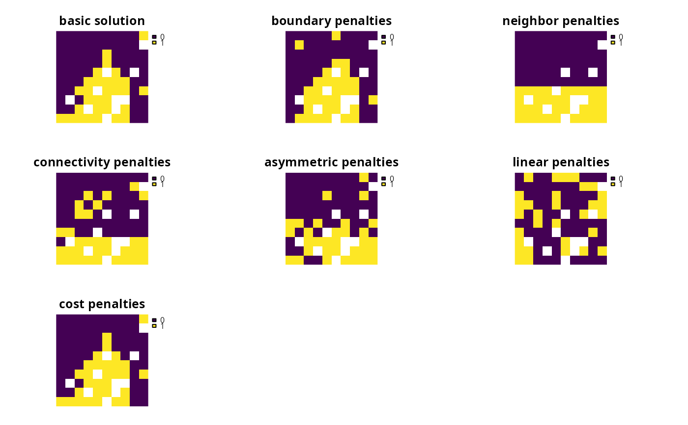
# plot solutions
plot(s, axes = FALSE)
# create problem with linear penalties, with a penalty scaling factor of 100
p6 <- p1 %>% add_linear_penalties(100, data = sim_penalty_raster)
# create problem with cost penalties, with a penalty scaling factor of 5
p7 <- p1 %>% add_cost_penalties(5)
# solve problems
s <- terra::rast(lapply(list(p1, p2, p3, p4, p5, p6, p7), solve))
names(s) <- c(
"basic solution", "boundary penalties", "neighbor penalties",
"connectivity penalties", "asymmetric penalties", "linear penalties",
"cost penalties"
)
# plot solutions
plot(s, axes = FALSE)