Conservation planning exercises rarely have access to all the data needed to identify the truly perfect solution. This is because available data may lack important details (e.g., land acquisition costs may be unavailable), contain errors (e.g., species presence/absence data may have false positives), or key objectives may not be formally incorporated into the prioritization process (e.g., future land use requirements). As such, conservation planners can help decision makers by providing them with a portfolio of solutions to inform their decision.
Details
The following functions can be used to add a portfolio to a
conservation planning problem(). Note that if multiple
of these functions are added to a problem(), then only the last
function added will be used.
add_default_portfolio()Generate a portfolio containing a single solution (per
add_single_portfolio()). This portfolio method is added toproblem()objects by default.add_single_portfolio()Generate a portfolio containing a single solution.
add_extra_portfolio()Generate a portfolio of solutions by storing feasible solutions found during the optimization process. This method is useful for quickly obtaining multiple solutions, but does not provide any guarantees on the number of solutions, or the quality of solutions. Note that it requires the Gurobi solver.
add_top_portfolio()Generate a portfolio of solutions by finding a pre-specified number of solutions that are closest to optimality (i.e., the top solutions). This is useful for examining differences among near-optimal solutions. It can also be used to generate multiple solutions and, in turn, to calculate selection frequencies for small problems. Note that it requires the Gurobi solver.
add_gap_portfolio()Generate a portfolio of solutions by finding a certain number of solutions that are all within a pre- specified optimality gap. Although this method may be useful for generating multiple solutions that can be used to calculate selection frequencies (similar to Marxan), note that this function tends to produce solutions that are very similar to each other and so you will (likely) need to generate thousands for solutions when calculating selection frequencies. Note that it requires the Gurobi solver.
add_cuts_portfolio()Generate a portfolio of distinct solutions within a pre-specified optimality gap using Bender's cuts. This is recommended as a replacement for
add_top_portfolio()when the Gurobi software is not available.add_shuffle_portfolio()Generate a portfolio of solutions by randomly reordering the data prior to attempting to solve the problem. This is recommended as a replacement for
add_gap_portfolio()when the Gurobi software is not available.
See also
Other overviews:
approaches,
constraints,
decisions,
importance,
objectives,
penalties,
solvers,
summaries,
targets
Examples
# load data
sim_pu_raster <- get_sim_pu_raster()
sim_features <- get_sim_features()
# create problem
p <-
problem(sim_pu_raster, sim_features) %>%
add_min_set_objective() %>%
add_relative_targets(0.1) %>%
add_binary_decisions() %>%
add_default_solver(gap = 0.02, verbose = FALSE)
# create problem with single portfolio
p1 <- p %>% add_single_portfolio()
# create problem with cuts portfolio with 4 solutions
p2 <- p %>% add_cuts_portfolio(4)
# create problem with shuffle portfolio with 4 solutions
p3 <- p %>% add_shuffle_portfolio(4)
# create problem with extra portfolio
p4 <- p %>% add_extra_portfolio()
# create problem with top portfolio with 4 solutions
p5 <- p %>% add_top_portfolio(4)
# create problem with gap portfolio with 4 solutions within 50% of optimality
p6 <- p %>% add_gap_portfolio(4, 0.5)
# solve problems to obtain solution portfolios
s <- list(solve(p1), solve(p2), solve(p3), solve(p4), solve(p5), solve(p6))
#> Generating solutions ■■■■■■■■■■■■■■■■ | 2/4 | 50% | ETA: 1s
#> Generating solutions ■■■■■■■■■■■■■■■■■■■■■■■■■■■■■■■ | 4/4 | 100% | ETA: 0s
# plot solution from default portfolio
plot(terra::rast(s[[1]]), axes = FALSE)
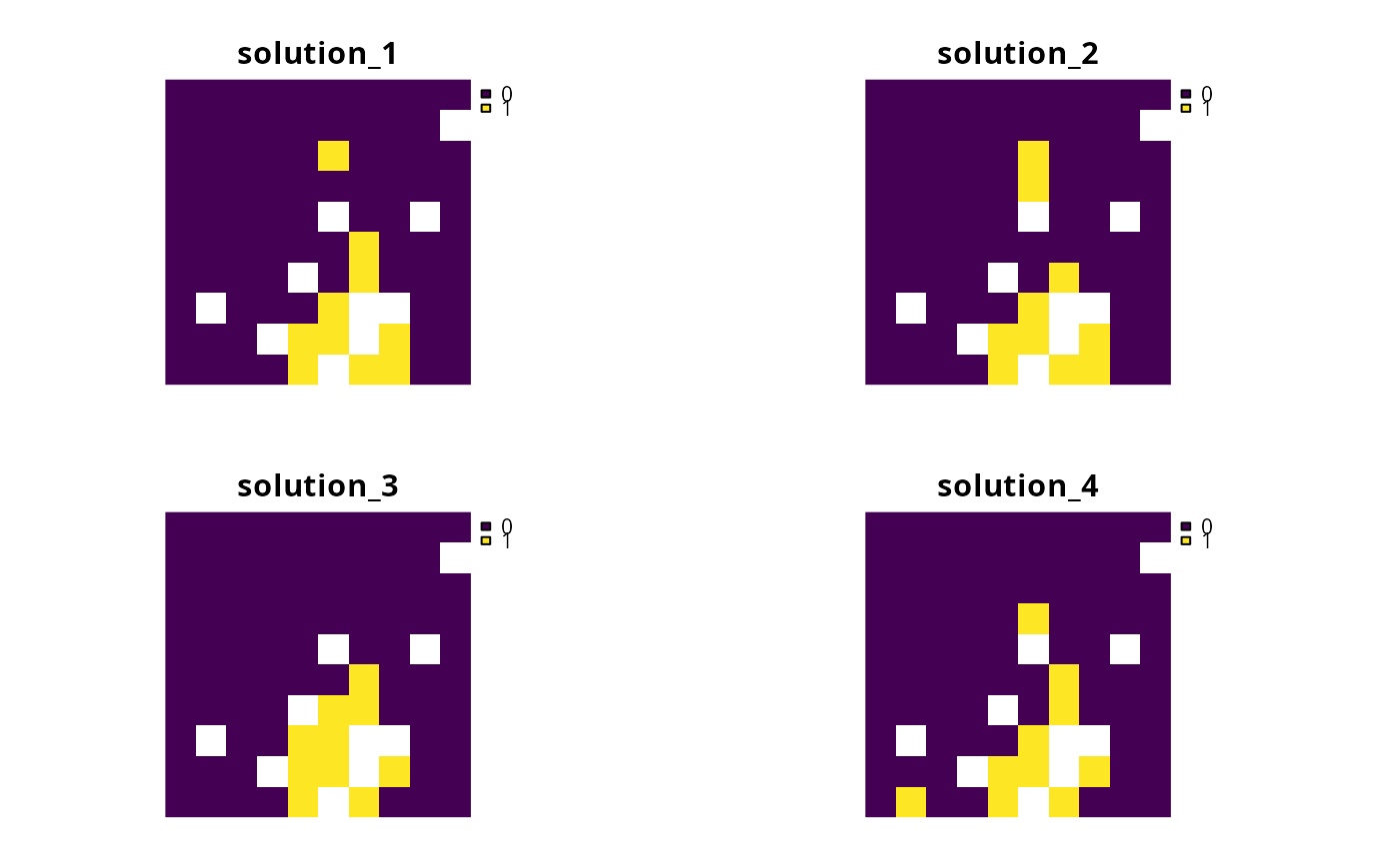
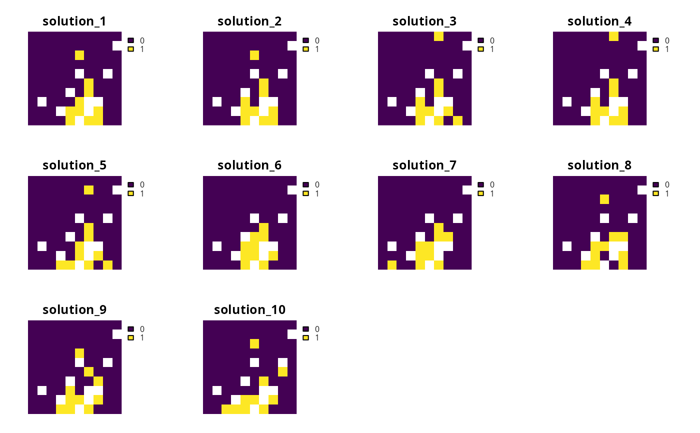
 # plot solutions from cuts portfolio
plot(terra::rast(s[[2]]), axes = FALSE)
# plot solutions from cuts portfolio
plot(terra::rast(s[[2]]), axes = FALSE)
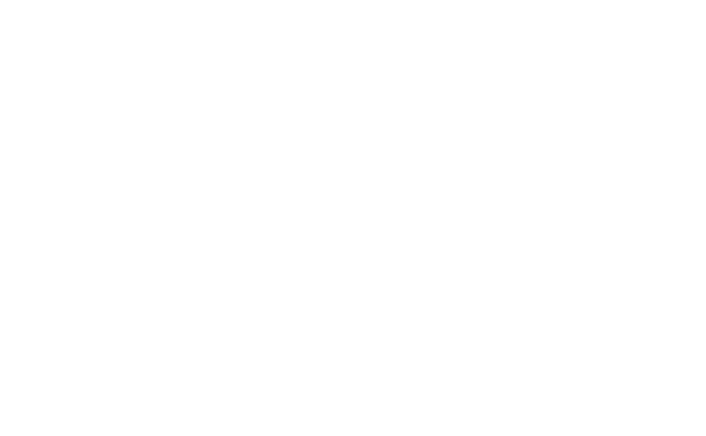
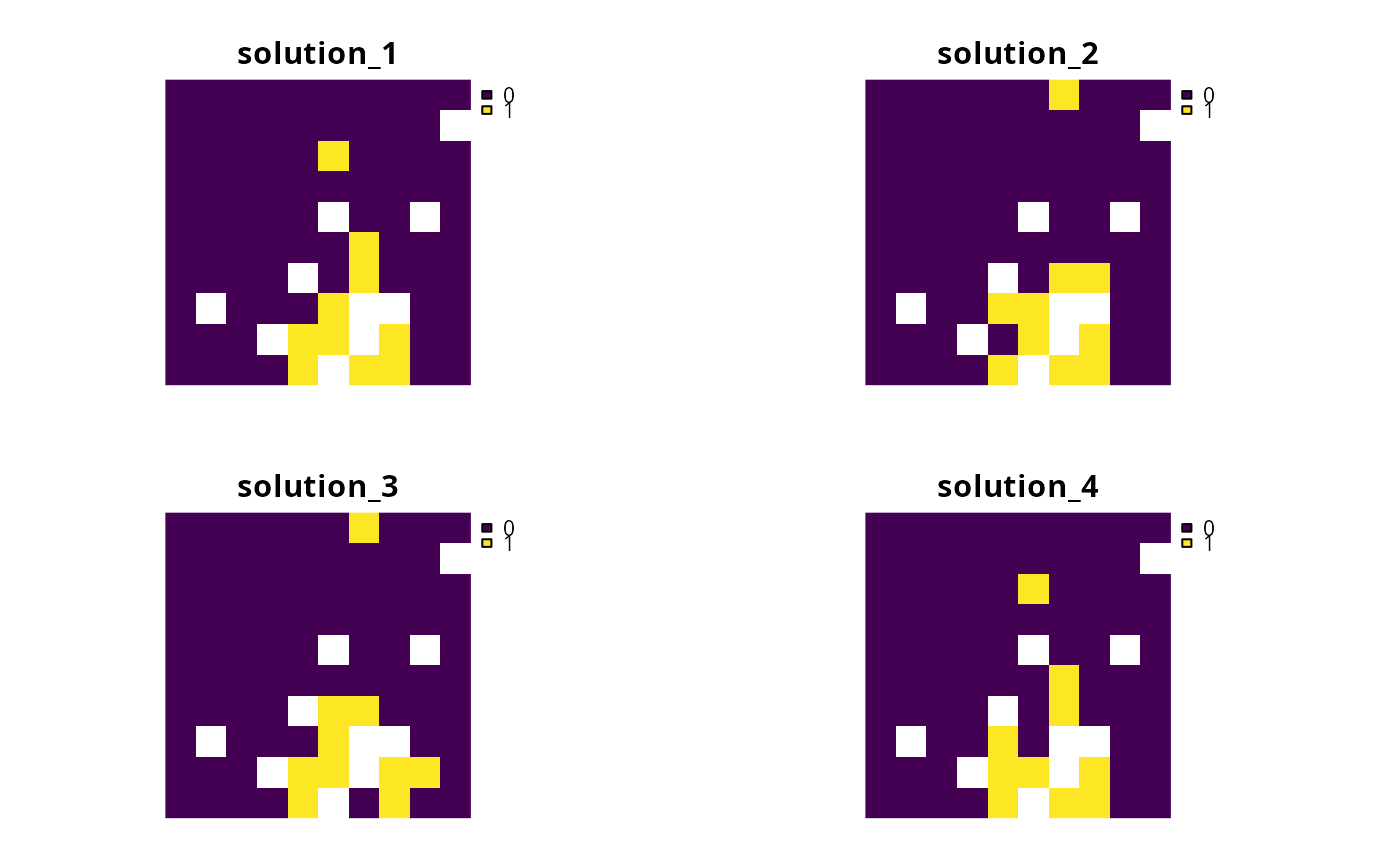
 # plot solutions from shuffle portfolio
plot(terra::rast(s[[3]]), axes = FALSE)
# plot solutions from shuffle portfolio
plot(terra::rast(s[[3]]), axes = FALSE)
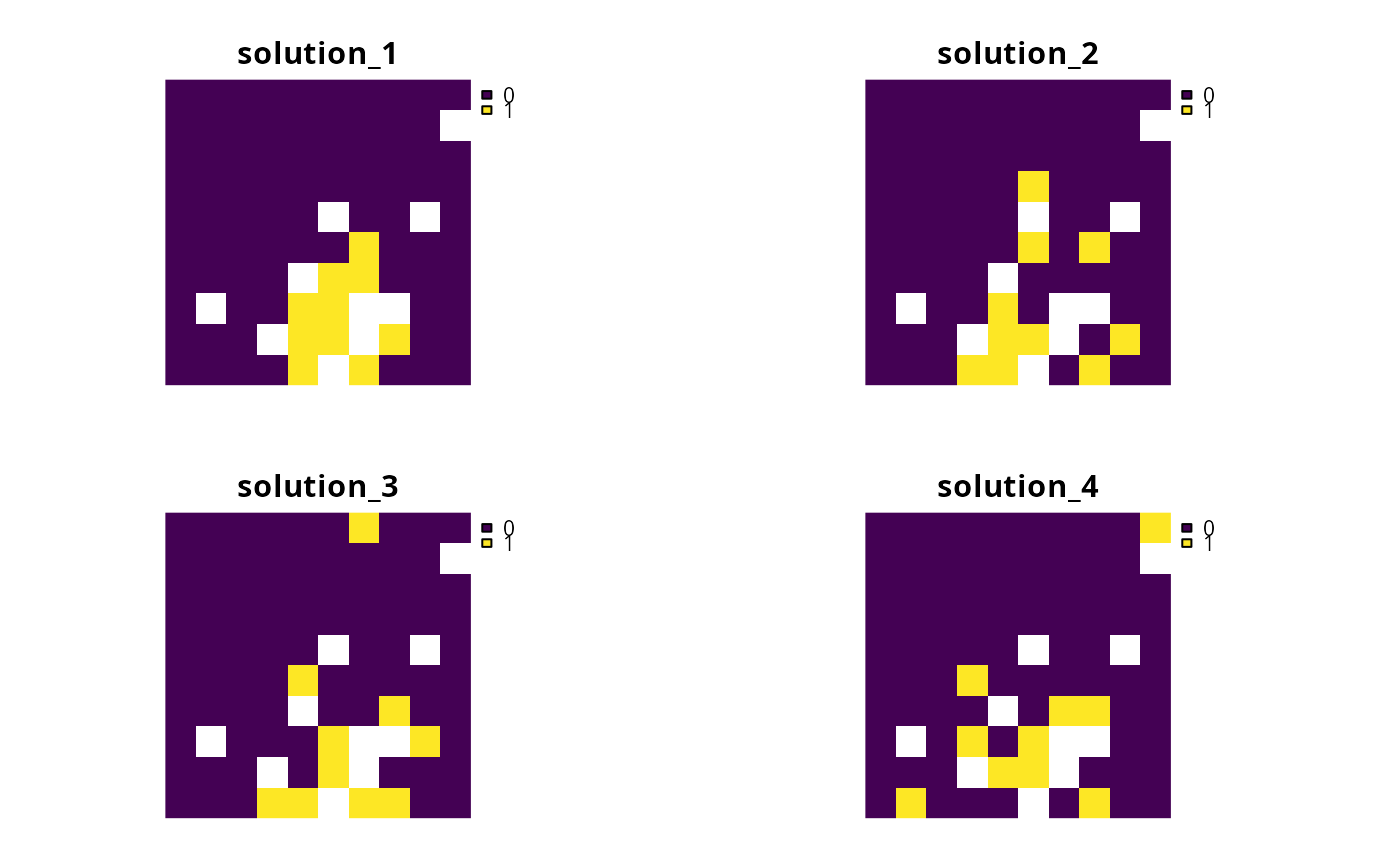
 # plot solutions from extra portfolio
plot(terra::rast(s[[4]]), axes = FALSE)
# plot solutions from extra portfolio
plot(terra::rast(s[[4]]), axes = FALSE)
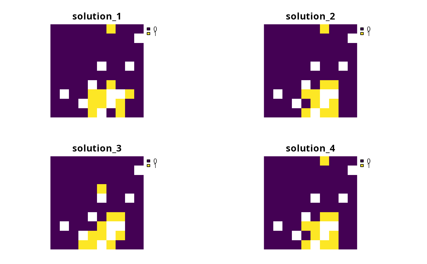
 # plot solutions from top portfolio
plot(terra::rast(s[[5]]), axes = FALSE)
# plot solutions from top portfolio
plot(terra::rast(s[[5]]), axes = FALSE)
 # plot solutions from gap portfolio
plot(terra::rast(s[[6]]), axes = FALSE)
# plot solutions from gap portfolio
plot(terra::rast(s[[6]]), axes = FALSE)