Generate a portfolio of solutions for a conservation planning problem by randomly reordering the data prior to solving the problem. Although this function can be useful for generating multiple different solutions for a given problem, it is recommended to use add_pool_portfolio if the Gurobi software is available.
Arguments
- x
problem()object.- number_solutions
integervalue denoting the number of required solutions. Defaults to 10.- threads
integervalue denoting the number of threads to use during optimization. Broadly speaking, we recommend settingthreadsto be no higher than the number of computational cores minus one or two (e.g.,threads = parallel::detectCores(TRUE) - 2). This is because settingthreadsto be equal to the number of computational cores means that the solver and is fighting for resources with other software (e.g., Dropbox, iCloud, OneDrive, software updates, antivirus software, internet browsers) and, in turn, can result in computational bottlenecks that slow run times. Additionally, when settingthreadsto be a value greater than 1, we recommend checking memory (RAM) usage during the optimization process to ensure that the solver does not use up the majority of available memory. This is because solving optimization problems with multiple threads can involve creating multiple copies of the problem (e.g.,threads = 5may mean 5 copies) and exhausting most of the available memory will drastically slow run times. Defaults to 1.- verbose
logicalshould progress on generating multiple solutions be displayed? Note that progress will not be displayed if using multiple threads for parallel processing. Defaults toTRUE.
Value
An updated problem() object with the portfolio added to it.
Details
This strategy for generating a portfolio of solutions often results in different solutions, depending on optimality gap, but may return duplicate solutions. In general, this strategy is most effective when problems are quick to solve and multiple threads are available for solving each problem separately.
Notes
In previous versions (< 9.0.0.0), this function had a remove_duplicates
parameter. To streamline and provide this functionality for other
functions, duplicate solutions can now be removed by using the
the remove_duplicates parameter of solve().
See also
Other functions for adding portfolios:
add_cuts_portfolio(),
add_default_portfolio(),
add_extra_portfolio(),
add_gap_portfolio(),
add_single_portfolio(),
add_top_portfolio()
Examples
# set seed for reproducibility
set.seed(500)
# load data
sim_pu_raster <- get_sim_pu_raster()
sim_features <- get_sim_features()
sim_zones_pu_raster <- get_sim_zones_pu_raster()
sim_zones_features <- get_sim_zones_features()
# create minimal problem with shuffle portfolio
p1 <-
problem(sim_pu_raster, sim_features) %>%
add_min_set_objective() %>%
add_relative_targets(0.2) %>%
add_shuffle_portfolio(10) %>%
add_default_solver(gap = 0.2, verbose = FALSE)
# solve problem and generate 10 solutions within 20% of optimality
s1 <- solve(p1)
#> Generating solutions ■■■■■■■■■■ | 3/10 | 30% | ETA: 3s
#> Generating solutions ■■■■■■■■■■■■■■■■■■■■■■■■■■■■ | 9/10 | 90% | ETA: 0s
#> Generating solutions ■■■■■■■■■■■■■■■■■■■■■■■■■■■■■■■ | 10/10 | 100% | ETA: 0s
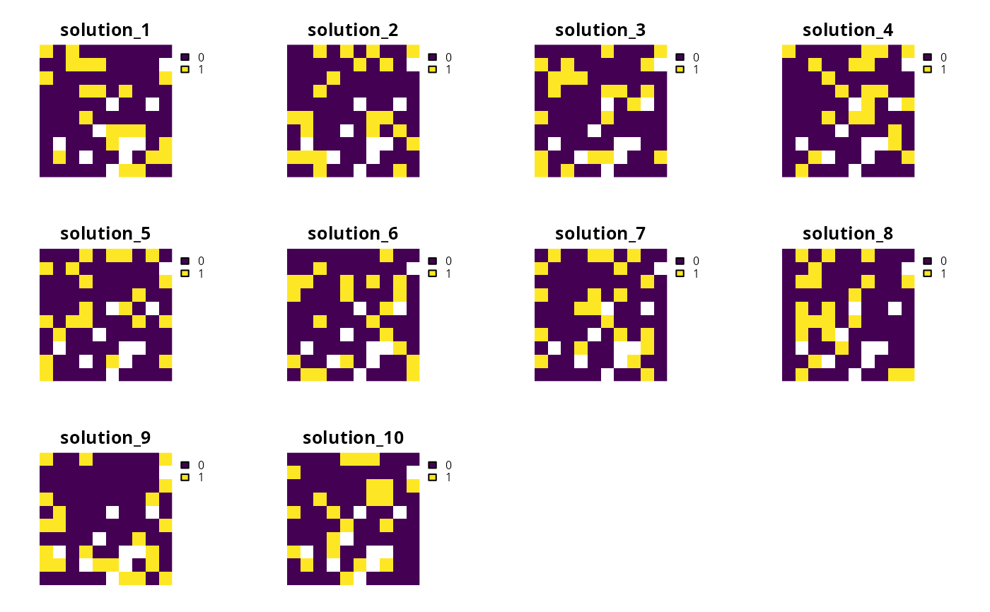
# convert portfolio into a multi-layer raster
s1 <- terra::rast(s1)
# print number of solutions found
print(terra::nlyr(s1))
#> [1] 10
# plot solutions in portfolio
plot(s1, axes = FALSE)
 # build multi-zone conservation problem with shuffle portfolio
p2 <-
problem(sim_zones_pu_raster, sim_zones_features) %>%
add_min_set_objective() %>%
add_relative_targets(matrix(runif(15, 0.1, 0.2), nrow = 5, ncol = 3)) %>%
add_binary_decisions() %>%
add_shuffle_portfolio(10) %>%
add_default_solver(gap = 0.2, verbose = FALSE)
# solve the problem
s2 <- solve(p2)
#> Generating solutions ■■■■■■■■■■■■■■■■■■■ | 6/10 | 60% | ETA: 2s
#> Generating solutions ■■■■■■■■■■■■■■■■■■■■■■■■■■■■■■■ | 10/10 | 100% | ETA: 0s
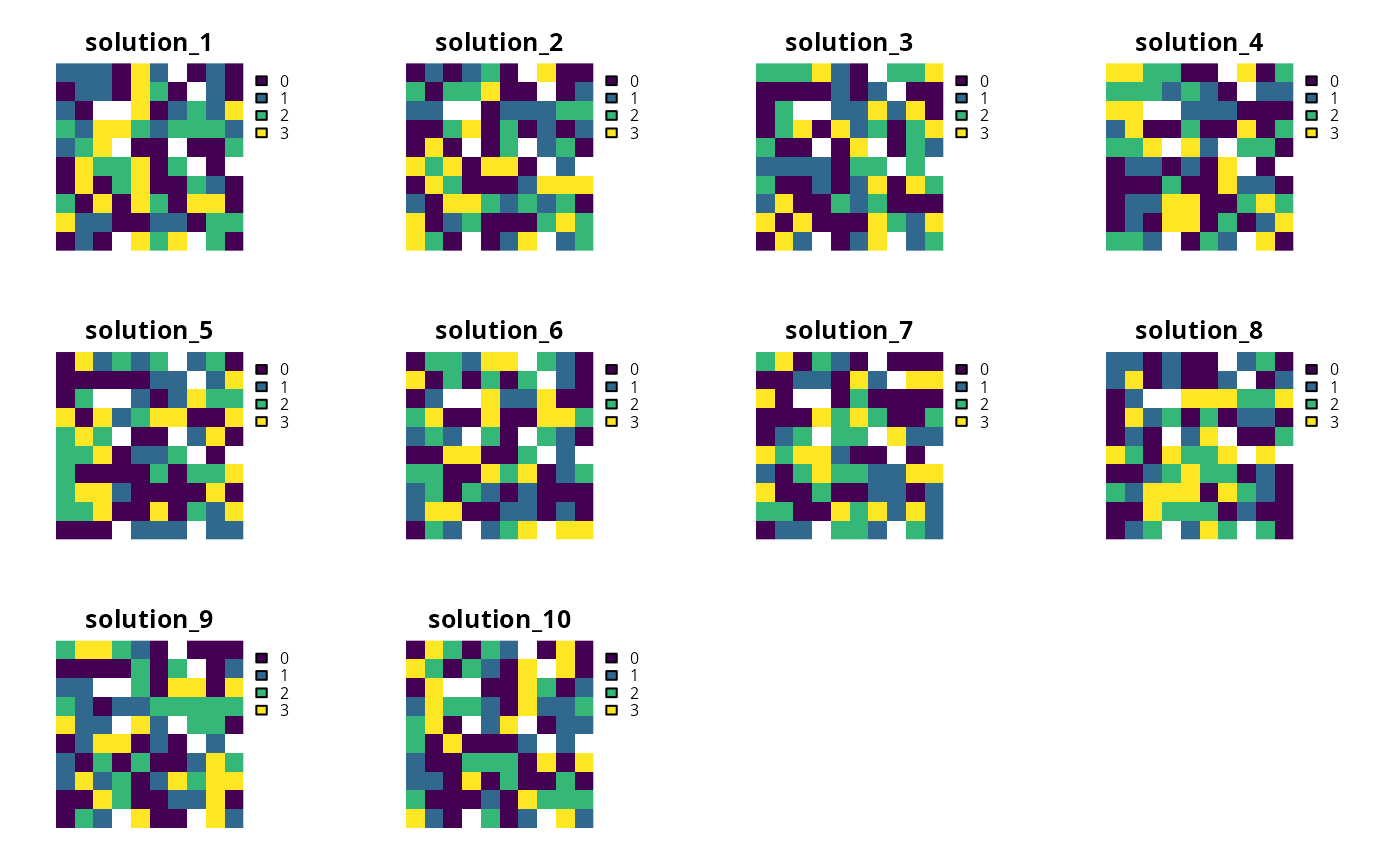
# convert each solution in the portfolio into a single category layer
s2 <- terra::rast(lapply(s2, category_layer))
# print number of solutions found
print(terra::nlyr(s2))
#> [1] 10
# plot solutions in portfolio
plot(s2, axes = FALSE)
# build multi-zone conservation problem with shuffle portfolio
p2 <-
problem(sim_zones_pu_raster, sim_zones_features) %>%
add_min_set_objective() %>%
add_relative_targets(matrix(runif(15, 0.1, 0.2), nrow = 5, ncol = 3)) %>%
add_binary_decisions() %>%
add_shuffle_portfolio(10) %>%
add_default_solver(gap = 0.2, verbose = FALSE)
# solve the problem
s2 <- solve(p2)
#> Generating solutions ■■■■■■■■■■■■■■■■■■■ | 6/10 | 60% | ETA: 2s
#> Generating solutions ■■■■■■■■■■■■■■■■■■■■■■■■■■■■■■■ | 10/10 | 100% | ETA: 0s
# convert each solution in the portfolio into a single category layer
s2 <- terra::rast(lapply(s2, category_layer))
# print number of solutions found
print(terra::nlyr(s2))
#> [1] 10
# plot solutions in portfolio
plot(s2, axes = FALSE)