Generate a portfolio of solutions for a conservation planning
problem using Bender's cuts (discussed in Rodrigues
et al. 2000). This is recommended as a replacement for
add_gap_portfolio() when the Gurobi software is not
available.
Arguments
- x
problem()object.- number_solutions
integervalue denoting the number of required solutions. Defaults to 10.- verbose
logicalshould progress on generating multiple solutions be displayed? Defaults toTRUE.
Value
An updated problem() object with the portfolio added to it.
Details
This strategy for generating a portfolio of solutions involves solving the problem multiple times and adding additional constraints to forbid previously obtained solutions. In general, this strategy is most useful when problems take a long time to solve and benefit from having multiple threads allocated for solving an individual problem.
Notes
In early versions (< 4.0.1), this function was only compatible with
Gurobi (i.e., add_gurobi_solver()). To provide functionality with
exact algorithm solvers, this function now adds constraints to the
problem formulation to generate multiple solutions.
References
Rodrigues AS, Cerdeira OJ, and Gaston KJ (2000) Flexibility, efficiency, and accountability: adapting reserve selection algorithms to more complex conservation problems. Ecography, 23: 565–574.
See also
See portfolios for an overview of all functions for adding a portfolio.
Other functions for adding portfolios:
add_default_portfolio(),
add_extra_portfolio(),
add_gap_portfolio(),
add_shuffle_portfolio(),
add_single_portfolio(),
add_top_portfolio()
Examples
# set seed for reproducibility
set.seed(500)
# load data
sim_pu_raster <- get_sim_pu_raster()
sim_features <- get_sim_features()
sim_zones_pu_raster <- get_sim_zones_pu_raster()
sim_zones_features <- get_sim_zones_features()
# create minimal problem with cuts portfolio
p1 <-
problem(sim_pu_raster, sim_features) %>%
add_min_set_objective() %>%
add_relative_targets(0.2) %>%
add_cuts_portfolio(10) %>%
add_default_solver(gap = 0.2, verbose = FALSE)
# solve problem and generate 10 solutions within 20% of optimality
s1 <- solve(p1)
#> Generating solutions ■■■■■■■■■■ | 3/10 | 30% | ETA: 3s
#> Generating solutions ■■■■■■■■■■■■■■■■ | 5/10 | 50% | ETA: 2s
#> Generating solutions ■■■■■■■■■■■■■■■■■■■■■■■■■■■■■■■ | 10/10 | 100% | ETA: 0s
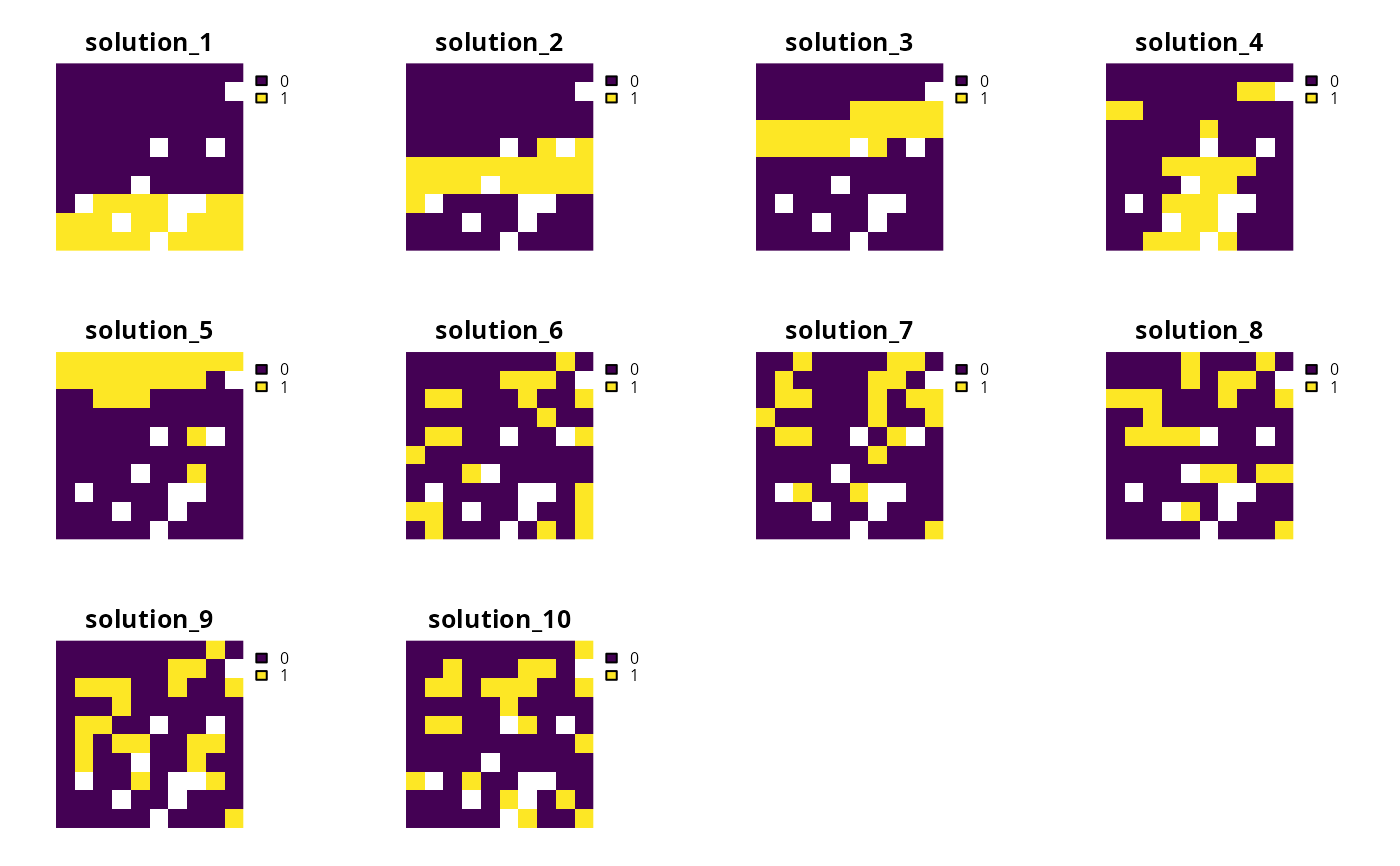
# convert portfolio into a multi-layer raster object
s1 <- terra::rast(s1)
# plot solutions in portfolio
plot(s1, axes = FALSE)
 # build multi-zone conservation problem with cuts portfolio
p2 <-
problem(sim_zones_pu_raster, sim_zones_features) %>%
add_min_set_objective() %>%
add_relative_targets(matrix(runif(15, 0.1, 0.2), nrow = 5, ncol = 3)) %>%
add_binary_decisions() %>%
add_cuts_portfolio(10) %>%
add_default_solver(gap = 0.2, verbose = FALSE)
# solve the problem
s2 <- solve(p2)
#> Generating solutions ■■■■■■■■■■ | 3/10 | 30% | ETA: 3s
#> Generating solutions ■■■■■■■■■■■■■■■■■■■■■■■■■■■■ | 9/10 | 90% | ETA: 0s
#> Generating solutions ■■■■■■■■■■■■■■■■■■■■■■■■■■■■■■■ | 10/10 | 100% | ETA: 0s
# print solution
str(s2, max.level = 1)
#> List of 10
#> $ solution_1 :S4 class 'SpatRaster' [package "terra"]
#> $ solution_2 :S4 class 'SpatRaster' [package "terra"]
#> $ solution_3 :S4 class 'SpatRaster' [package "terra"]
#> $ solution_4 :S4 class 'SpatRaster' [package "terra"]
#> $ solution_5 :S4 class 'SpatRaster' [package "terra"]
#> $ solution_6 :S4 class 'SpatRaster' [package "terra"]
#> $ solution_7 :S4 class 'SpatRaster' [package "terra"]
#> $ solution_8 :S4 class 'SpatRaster' [package "terra"]
#> $ solution_9 :S4 class 'SpatRaster' [package "terra"]
#> $ solution_10:S4 class 'SpatRaster' [package "terra"]
#> - attr(*, "objective")= Named num [1:10] 12615 12312 12381 12404 12173 ...
#> ..- attr(*, "names")= chr [1:10] "solution_1" "solution_2" "solution_3" "solution_4" ...
#> - attr(*, "status")= Named chr [1:10] "OPTIMAL" "OPTIMAL" "OPTIMAL" "OPTIMAL" ...
#> ..- attr(*, "names")= chr [1:10] "solution_1" "solution_2" "solution_3" "solution_4" ...
#> - attr(*, "runtime")= Named num [1:10] 0.006 0.005 0.005 0.006 0.005 ...
#> ..- attr(*, "names")= chr [1:10] "solution_1" "solution_2" "solution_3" "solution_4" ...
#> - attr(*, "gap")= Named num [1:10] 0.175 0.183 0.187 0.189 0.173 ...
#> ..- attr(*, "names")= chr [1:10] "solution_1" "solution_2" "solution_3" "solution_4" ...
#> - attr(*, "objbound")= Named num [1:10] 0.175 0.183 0.187 0.189 0.173 ...
#> ..- attr(*, "names")= chr [1:10] "solution_1" "solution_2" "solution_3" "solution_4" ...
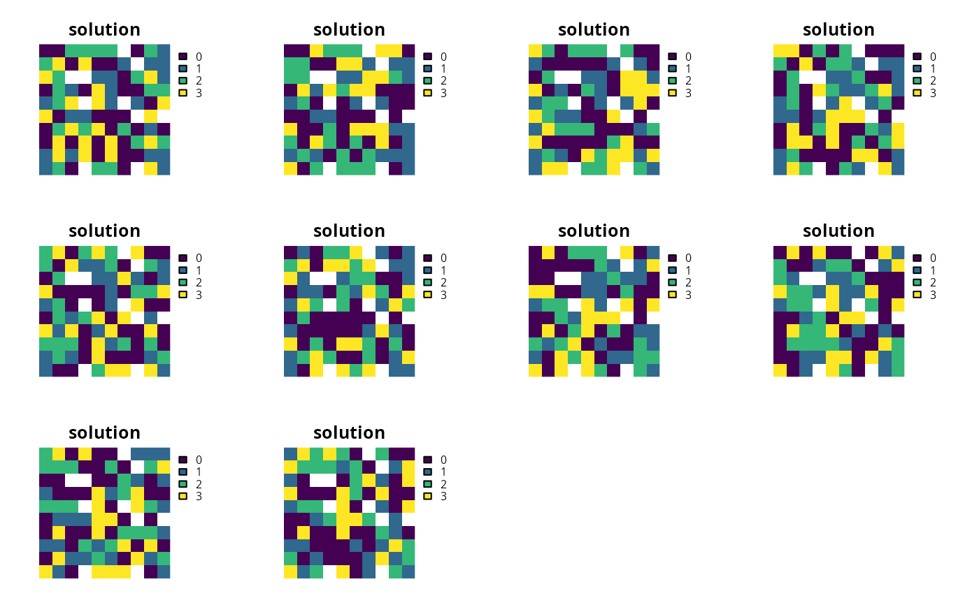
# convert each solution in the portfolio into a single category layer
s2 <- terra::rast(lapply(s2, category_layer))
# plot solutions in portfolio
plot(s2, main = "solution", axes = FALSE)
# build multi-zone conservation problem with cuts portfolio
p2 <-
problem(sim_zones_pu_raster, sim_zones_features) %>%
add_min_set_objective() %>%
add_relative_targets(matrix(runif(15, 0.1, 0.2), nrow = 5, ncol = 3)) %>%
add_binary_decisions() %>%
add_cuts_portfolio(10) %>%
add_default_solver(gap = 0.2, verbose = FALSE)
# solve the problem
s2 <- solve(p2)
#> Generating solutions ■■■■■■■■■■ | 3/10 | 30% | ETA: 3s
#> Generating solutions ■■■■■■■■■■■■■■■■■■■■■■■■■■■■ | 9/10 | 90% | ETA: 0s
#> Generating solutions ■■■■■■■■■■■■■■■■■■■■■■■■■■■■■■■ | 10/10 | 100% | ETA: 0s
# print solution
str(s2, max.level = 1)
#> List of 10
#> $ solution_1 :S4 class 'SpatRaster' [package "terra"]
#> $ solution_2 :S4 class 'SpatRaster' [package "terra"]
#> $ solution_3 :S4 class 'SpatRaster' [package "terra"]
#> $ solution_4 :S4 class 'SpatRaster' [package "terra"]
#> $ solution_5 :S4 class 'SpatRaster' [package "terra"]
#> $ solution_6 :S4 class 'SpatRaster' [package "terra"]
#> $ solution_7 :S4 class 'SpatRaster' [package "terra"]
#> $ solution_8 :S4 class 'SpatRaster' [package "terra"]
#> $ solution_9 :S4 class 'SpatRaster' [package "terra"]
#> $ solution_10:S4 class 'SpatRaster' [package "terra"]
#> - attr(*, "objective")= Named num [1:10] 12615 12312 12381 12404 12173 ...
#> ..- attr(*, "names")= chr [1:10] "solution_1" "solution_2" "solution_3" "solution_4" ...
#> - attr(*, "status")= Named chr [1:10] "OPTIMAL" "OPTIMAL" "OPTIMAL" "OPTIMAL" ...
#> ..- attr(*, "names")= chr [1:10] "solution_1" "solution_2" "solution_3" "solution_4" ...
#> - attr(*, "runtime")= Named num [1:10] 0.006 0.005 0.005 0.006 0.005 ...
#> ..- attr(*, "names")= chr [1:10] "solution_1" "solution_2" "solution_3" "solution_4" ...
#> - attr(*, "gap")= Named num [1:10] 0.175 0.183 0.187 0.189 0.173 ...
#> ..- attr(*, "names")= chr [1:10] "solution_1" "solution_2" "solution_3" "solution_4" ...
#> - attr(*, "objbound")= Named num [1:10] 0.175 0.183 0.187 0.189 0.173 ...
#> ..- attr(*, "names")= chr [1:10] "solution_1" "solution_2" "solution_3" "solution_4" ...
# convert each solution in the portfolio into a single category layer
s2 <- terra::rast(lapply(s2, category_layer))
# plot solutions in portfolio
plot(s2, main = "solution", axes = FALSE)