Add linear penalties

Add penalties to a conservation planning problem to penalize solutions that select planning units with higher values from a specific data source (e.g., anthropogenic impact). These penalties assume a linear trade-off between the penalty values and the primary objective of the conservation planning problem (e.g., solution cost for minimum set problems; add_min_set_objective().

Usage

# S4 method for class 'ConservationProblem,ANY,character'
add_linear_penalties(x, penalty, data)

# S4 method for class 'ConservationProblem,ANY,numeric'
add_linear_penalties(x, penalty, data)

# S4 method for class 'ConservationProblem,ANY,matrix'
add_linear_penalties(x, penalty, data)

# S4 method for class 'ConservationProblem,ANY,Matrix'
add_linear_penalties(x, penalty, data)

# S4 method for class 'ConservationProblem,ANY,Raster'
add_linear_penalties(x, penalty, data)

# S4 method for class 'ConservationProblem,ANY,SpatRaster'
add_linear_penalties(x, penalty, data)

# S4 method for class 'ConservationProblem,ANY,dgCMatrix'
add_linear_penalties(x, penalty, data)

Arguments

x: problem() object.
penalty: numeric value denoting the importance of not selecting planning units with high data values. Higher penalty values can be used to obtain solutions that are strongly averse to selecting places with high data values, and smaller penalty values can be used to obtain solutions that only avoid places with especially high data values. Note that negative penalty values can be used to obtain solutions that prefer places with high data values. Additionally, if has x has multiple zones, then penalty must have a value for each zone.
data: character, numeric, terra::rast(), matrix, or Matrix object containing the values used to penalize solutions. Planning units that are associated with higher data values are penalized more strongly in the solution. See the Data format section for more information.

Value

An updated problem() object with the penalties added to it.

Details

This function penalizes solutions that have higher values according to the sum of the penalty values associated with each planning unit, weighted by status of each planning unit in the solution.

Data format

The following formats can be used to specify data.

data as a character vector: Here values are specified based on column name(s) for the planning unit data in x. This format is only compatible if the planning units in x are a sf::sf() or data.frame object. The column(s) must have numeric values, and must not contain any missing (NA) values. If x has a single zone, then data must contain a single column name. Otherwise, if x has multiple zones, then data must contain a column name for each zone.
data as a numeric vector: Here values are specified for each planning unit. These values must not contain any missing (NA) values. Note that this format can only be used if x has a single zone.
data as a matrix/Matrix object: Here values are specified for each planning unit and each zone. Note that data must have numeric values. Each row corresponds to a planning unit, each column corresponds to a zone, and each cell indicates the value associated with a planning unit when it is allocated to a given zone.
data as a terra::rast() object: Here values are specified for each planning unit and each zone. This format is only compatible if the planning units in x are sf::sf(), or terra::rast() objects. If the planning unit data are a sf::sf() object, then the values are calculated by overlaying the planning units with data and calculating the sum of the values associated with each planning unit. If the planning unit data are a terra::rast() object, then the values are calculated by extracting the cell values (note that data and the planning unit in x must have exactly the same dimensionality, extent, and missing values). Additionally, if x has multiple zones, then data must contain a layer for each zone.

Mathematical formulation

The linear penalties are implemented using the following equations. Let $I$ denote the set of planning units (indexed by $i$), $Z$ the set of management zones (indexed by $z$), and $X_{iz}$ the decision variable for allocating planning unit $i$ to zone $z$ (e.g., with binary values indicating if each planning unit is allocated or not). Also, let $P_z$ represent the penalty scaling value for zones $z \in Z$ (per penalty), and $D_{iz}$ represent the penalty data for allocating planning unit $i \in I$ to zones $z \in Z$ (per data in matrix format).

$$ \sum_{i}^{I} \sum_{z}^{Z} P_z \times D_{iz} \times X_{iz} $$

Note that when the problem objective is to maximize some measure of benefit and not minimize some measure of cost, the term $P_z$ is replaced with $-P_z$.

Examples

# set seed for reproducibility
set.seed(600)

# load data
sim_pu_polygons <- get_sim_pu_polygons()
sim_features <- get_sim_features()
sim_zones_pu_raster <- get_sim_zones_pu_raster()
sim_zones_features <- get_sim_zones_features()

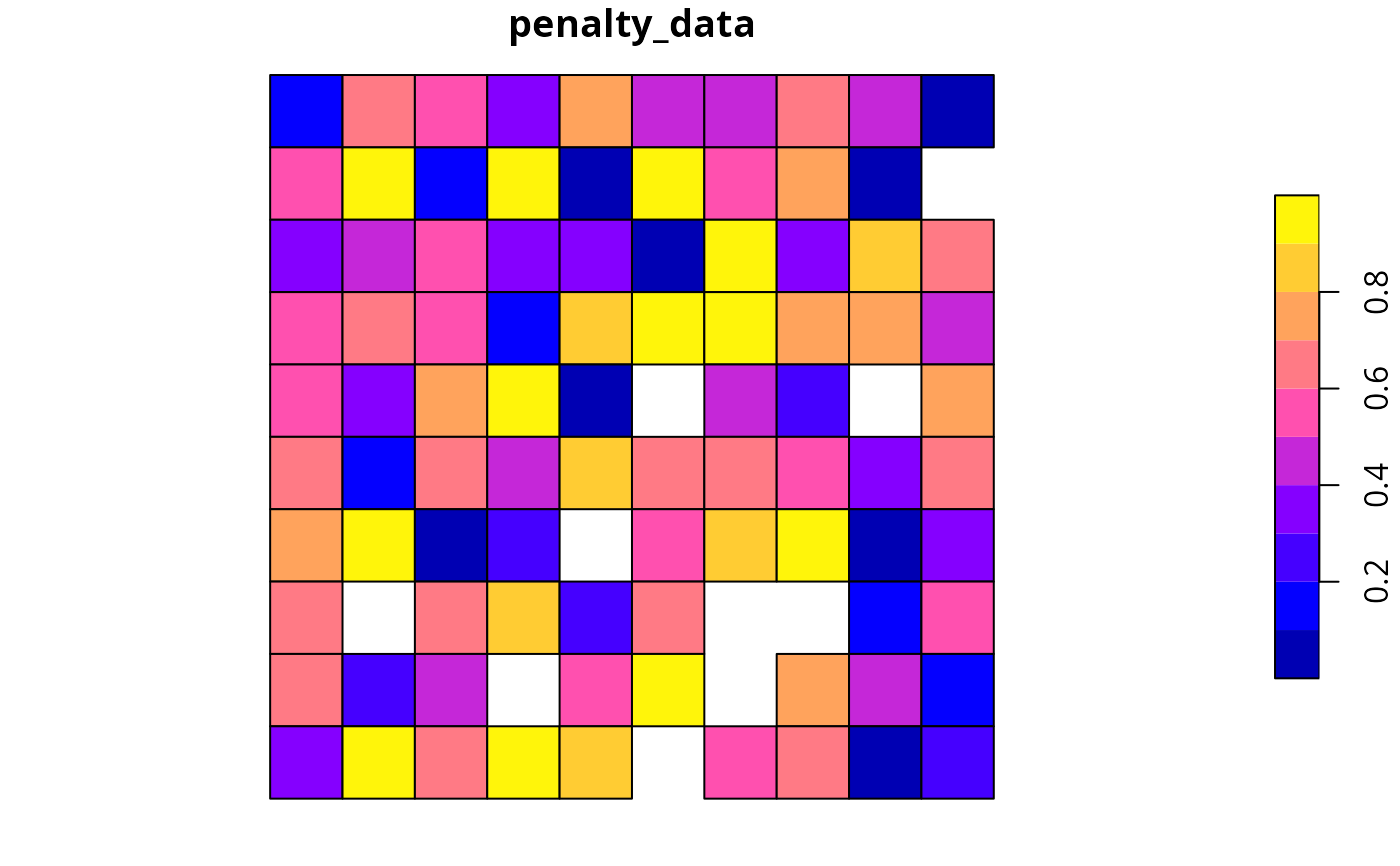
# add a column to contain the penalty data for each planning unit
# e.g., these values could indicate the level of habitat
sim_pu_polygons$penalty_data <- runif(nrow(sim_pu_polygons))

# plot the penalty data to visualise its spatial distribution
plot(sim_pu_polygons[, "penalty_data"], axes = FALSE)


# create minimal problem with minimum set objective,
# this does not use the penalty data
p1 <-
  problem(sim_pu_polygons, sim_features, cost_column = "cost") %>%
  add_min_set_objective() %>%
  add_relative_targets(0.1) %>%
  add_binary_decisions() %>%
  add_default_solver(verbose = FALSE)

# print problem
print(p1)
#> A conservation problem (<ConservationProblem>)
#> ├•data
#> │├•features:    "feature_1", "feature_2", "feature_3", … (5 total)
#> │└•planning units:
#> │ ├•data:       <sf> (90 total)
#> │ ├•costs:      continuous values (between 190.1328 and 215.8638)
#> │ ├•extent:     0, 0, 1, 1 (xmin, ymin, xmax, ymax)
#> │ └•CRS:        WGS 84 / Pseudo-Mercator (projected)
#> ├•formulation
#> │├•objective:   minimum set objective
#> │├•penalties:   none specified
#> │├•features:
#> ││├•targets:    relative targets (all equal to 0.1)
#> ││└•weights:    none specified
#> │├•constraints: none specified
#> │└•decisions:   binary decision
#> └•optimization
#>  ├•portfolio:   single portfolio
#>  └•solver:      gurobi solver (`gap` = 0.1, `time_limit` = 2147483647, …)
#> # ℹ Use `summary(...)` to see further details.

# create an updated version of the previous problem,
# with the penalties added to it
p2 <- p1 %>% add_linear_penalties(100, data = "penalty_data")

# print problem
print(p2)
#> A conservation problem (<ConservationProblem>)
#> ├•data
#> │├•features:    "feature_1", "feature_2", "feature_3", … (5 total)
#> │└•planning units:
#> │ ├•data:       <sf> (90 total)
#> │ ├•costs:      continuous values (between 190.1328 and 215.8638)
#> │ ├•extent:     0, 0, 1, 1 (xmin, ymin, xmax, ymax)
#> │ └•CRS:        WGS 84 / Pseudo-Mercator (projected)
#> ├•formulation
#> │├•objective:   minimum set objective
#> │├•penalties: 
#> ││└•1:          linear penalties (`penalty` = 100, …)
#> │├•features:
#> ││├•targets:    relative targets (all equal to 0.1)
#> ││└•weights:    none specified
#> │├•constraints: none specified
#> │└•decisions:   binary decision
#> └•optimization
#>  ├•portfolio:   single portfolio
#>  └•solver:      gurobi solver (`gap` = 0.1, `time_limit` = 2147483647, …)
#> # ℹ Use `summary(...)` to see further details.

# solve the two problems
s1 <- solve(p1)
s2 <- solve(p2)

# create a new object with both solutions
s3 <- sf::st_sf(
  tibble::tibble(
    s1 = s1$solution_1,
    s2 = s2$solution_1
  ),
  geometry = sf::st_geometry(s1)
)


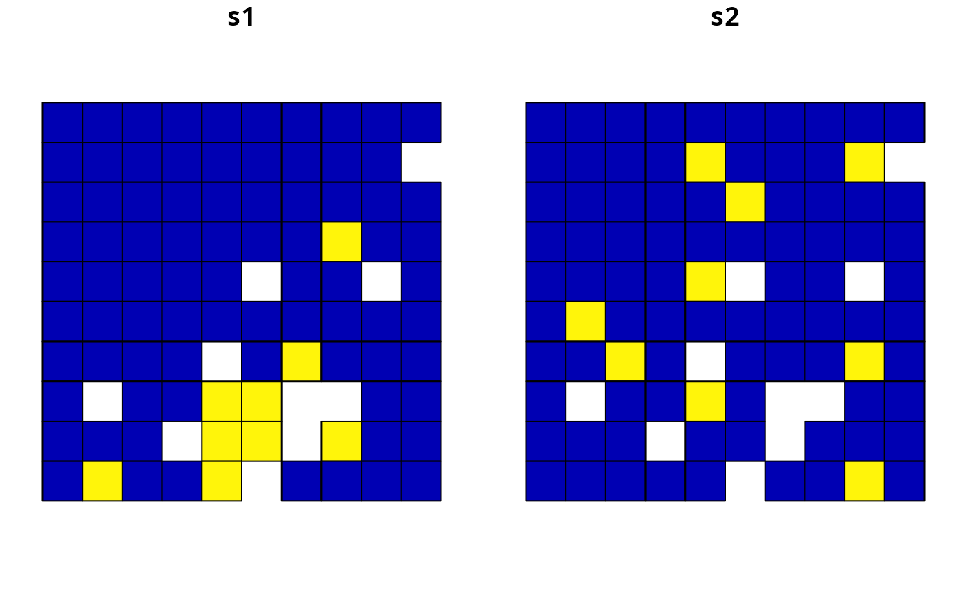
# plot the solutions and compare them,
# since we supplied a very high penalty value (i.e., 100), relative
# to the range of values in the penalty data and the objective function,
# the solution in s2 is very sensitive to values in the penalty data
plot(s3, axes = FALSE)


# for real conservation planning exercises,
# it would be worth exploring a range of penalty values (e.g., ranging
# from 1 to 100 increments of 5) to explore the trade-offs

# now, let's examine a conservation planning exercise involving multiple
# management zones

# create targets for each feature within each zone,
# these targets indicate that each zone needs to represent 10% of the
# spatial distribution of each feature
targ <- matrix(
  0.1, ncol = number_of_zones(sim_zones_features),
  nrow = number_of_features(sim_zones_features)
)

# create penalty data for allocating each planning unit to each zone,
# these data will be generated by simulating values
penalty_raster <- simulate_cost(
  sim_zones_pu_raster[[1]],
  n = number_of_zones(sim_zones_features)
)

# plot the penalty data, each layer corresponds to a different zone
plot(penalty_raster, main = "penalty data", axes = FALSE)


# create a multi-zone problem with the minimum set objective
# and penalties for allocating planning units to each zone,
# with a penalty scaling factor of 1 for each zone
p4 <-
  problem(sim_zones_pu_raster, sim_zones_features) %>%
  add_min_set_objective() %>%
  add_relative_targets(targ) %>%
  add_linear_penalties(c(1, 1, 1), penalty_raster) %>%
  add_binary_decisions() %>%
  add_default_solver(verbose = FALSE)

# print problem
print(p4)
#> A conservation problem (<ConservationProblem>)
#> ├•data
#> │├•zones:       "zone_1", "zone_2", and "zone_3" (3 total)
#> │├•features:    "feature_1", "feature_2", "feature_3", … (5 total)
#> │└•planning units:
#> │ ├•data:       <SpatRaster> (90 total)
#> │ ├•costs:      continuous values (between 182.6017 and 224.8492)
#> │ ├•extent:     0, 0, 1, 1 (xmin, ymin, xmax, ymax)
#> │ └•CRS:        WGS 84 / Pseudo-Mercator (projected)
#> ├•formulation
#> │├•objective:   minimum set objective
#> │├•penalties: 
#> ││└•1:          linear penalties (`penalty` = 1, 1, and 1, …)
#> │├•features:
#> ││├•targets:    relative targets (all equal to 0.1)
#> ││└•weights:    none specified
#> │├•constraints: none specified
#> │└•decisions:   binary decision
#> └•optimization
#>  ├•portfolio:   single portfolio
#>  └•solver:      gurobi solver (`gap` = 0.1, `time_limit` = 2147483647, …)
#> # ℹ Use `summary(...)` to see further details.

# solve problem
s4 <- solve(p4)

# plot solution
plot(category_layer(s4), main = "multi-zone solution", axes = FALSE)