Add feature weights

Add features weights to a conservation planning problem. Specifically, some objective functions aim to maximize (or minimize) a metric that evaluates how well a set of features are represented by a solution (e.g., maximize the number of feature targets that are met, add_max_n_targets_met_objective()). In such cases, it may be desirable to prefer the representation of some features over other features (e.g., features that have higher extinction risk might be considered more important than those with lower extinction risk). To achieve this, weights can be used to specify how much more important it is for a solution to represent particular features compared with other features.

Usage

# S4 method for class 'ConservationProblem,numeric'
add_feature_weights(x, weights)

# S4 method for class 'ConservationProblem,matrix'
add_feature_weights(x, weights)

Arguments

x: problem() object.
weights: numeric vector or matrix of weights. See the Weights format section for more information.

Value

An updated problem() with the weights added to it.

Details

Weights are only considered during optimization if a budget-limited objective is specified (e.g., add_max_cover_objective(), add_min_shortfall_objective()). Although weights can be added to problems that have the minimum set objective (i.e., add_min_set_objective()), they will have no effect during optimization and a warning will be thrown.

Weights format

The following formats can be used to specify weights. Note that weights must have values that are greater than, or equal to, zero (in other words, non-negative values).

weights as a numeric vector: Here weight values are specified for each feature. Note that this format cannot be used if x has multiple zones.
weights as a matrix object: Here weight values are specified for each feature in each zone. In particular, each row corresponds to a different feature in x, each column corresponds to a different zone in x, and cell values specify the weight value for representing a particular feature in a particular zone. Note that if the problem contains targets created using add_manual_targets(), then weights should be a matrix that has a single column containing the weight value for meeting each target.

Examples

# load package
require(ape)
#> Loading required package: ape

# load data
sim_pu_raster <- get_sim_pu_raster()
sim_features <- get_sim_features()
sim_phylogeny <- get_sim_phylogeny()
sim_zones_pu_raster <- get_sim_zones_pu_raster()
sim_zones_features <- get_sim_zones_features()

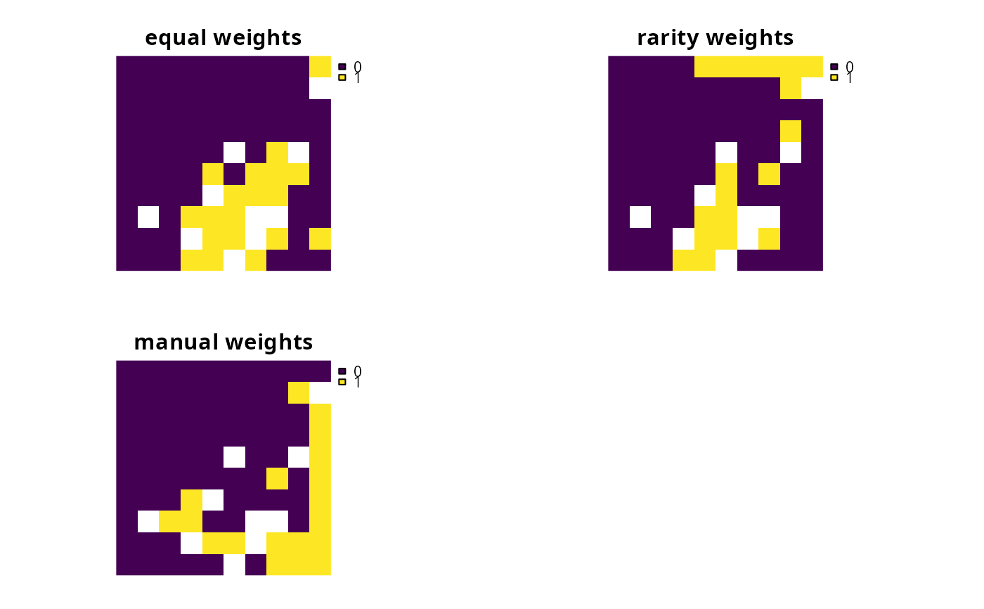
# create minimal problem that aims to maximize the number of features
# adequately conserved given a total budget of 3800. Here, each feature
# needs 20% of its habitat for it to be considered adequately conserved
p1 <-
  problem(sim_pu_raster, sim_features) %>%
  add_max_n_targets_met_objective(budget = 3800) %>%
  add_relative_targets(0.2) %>%
  add_binary_decisions() %>%
  add_default_solver(verbose = FALSE)

# create weights that assign higher importance to features with less
# suitable habitat in the study area
w2 <- exp((1 / terra::global(sim_features, "sum", na.rm = TRUE)[[1]]) * 200)

# create problem using rarity weights
p2 <- p1 %>% add_feature_weights(w2)

# create manually specified weights that assign higher importance to
# certain features. These weights could be based on a pre-calculated index
# (e.g., an index measuring extinction risk where higher values
# denote higher extinction risk)
w3 <- c(0, 0, 0, 100, 200)
p3 <- p1 %>% add_feature_weights(w3)

# solve problems
s1 <- c(solve(p1), solve(p2), solve(p3))
names(s1) <- c("equal weights", "rarity weights", "manual weights")

# plot solutions
plot(s1, axes = FALSE)


# plot the example phylogeny
par(mfrow = c(1, 1))
plot(sim_phylogeny, main = "simulated phylogeny")


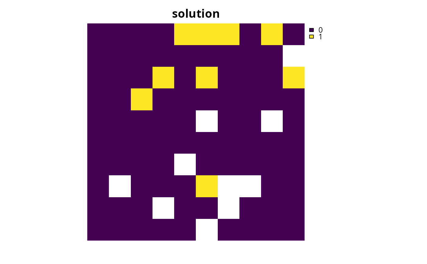
# create problem with a maximum phylogenetic diversity objective,
# where each feature needs 10% of its distribution to be secured for
# it to be adequately conserved and a total budget of 1900
p4 <-
  problem(sim_pu_raster, sim_features) %>%
  add_max_phylo_div_objective(1900, sim_phylogeny) %>%
  add_relative_targets(0.1) %>%
  add_binary_decisions() %>%
  add_default_solver(verbose = FALSE)

# solve problem
s4 <- solve(p4)

# plot solution
plot(s4, main = "solution", axes = FALSE)


# find out which features have their targets met
r4 <- eval_target_coverage_summary(p4, s4)
print(r4, width = Inf)
#> # A tibble: 5 × 10
#>   feature   met   total_amount absolute_target absolute_held absolute_shortfall
#>   <chr>     <lgl>        <dbl>           <dbl>         <dbl>              <dbl>
#> 1 feature_1 FALSE         83.3            8.33          6.84              1.49 
#> 2 feature_2 TRUE          31.2            3.12          3.24              0    
#> 3 feature_3 FALSE         72.0            7.20          6.02              1.18 
#> 4 feature_4 TRUE          42.7            4.27          4.31              0    
#> 5 feature_5 FALSE         56.7            5.67          4.70              0.973
#>   relative_target relative_held relative_shortfall relative_met
#>             <dbl>         <dbl>              <dbl>        <dbl>
#> 1             0.1        0.0821              0.179        0.821
#> 2             0.1        0.104               0            1    
#> 3             0.1        0.0836              0.164        0.836
#> 4             0.1        0.101               0            1    
#> 5             0.1        0.0828              0.172        0.828

# plot the example phylogeny and color the represented features in red
plot(
  sim_phylogeny, main = "represented features",
  tip.color = replace(
    rep("black", terra::nlyr(sim_features)), which(r4$met), "red"
  )
)


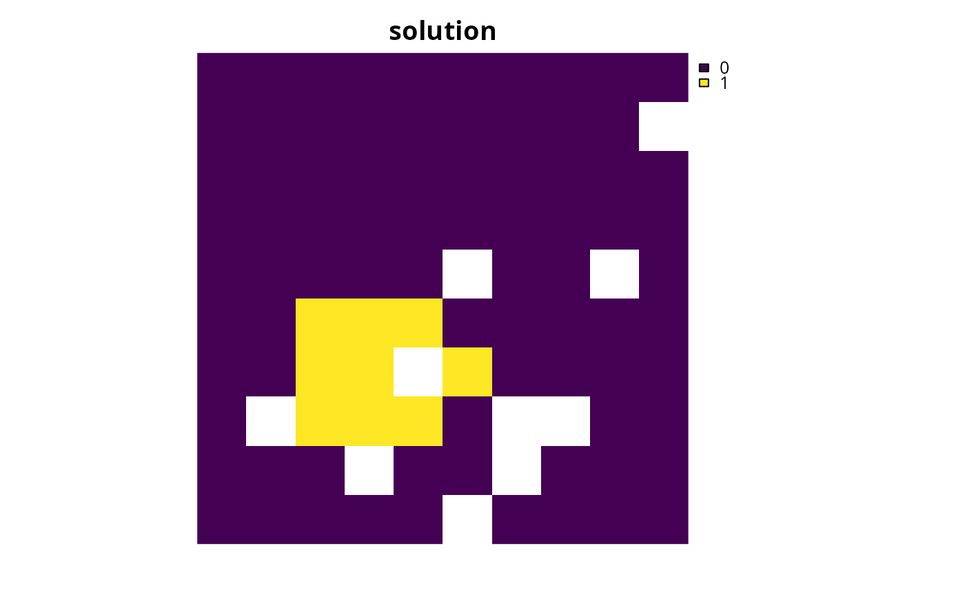
# we can see here that the third feature ("layer.3", i.e.,
# sim_features[[3]]) is not represented in the solution. Let us pretend
# that it is absolutely critical this feature is adequately conserved
# in the solution. For example, this feature could represent a species
# that plays important role in the ecosystem, or a species that is
# important commercial activities (e.g., eco-tourism). So, to generate
# a solution that conserves the third feature whilst also aiming to
# maximize phylogenetic diversity, we will create a set of weights that
# assign a particularly high weighting to the third feature
w5 <- c(0, 0, 10000, 0, 0)

# we can see that this weighting (i.e., w5[3]) has a much higher value than
# the branch lengths in the phylogeny so solutions that represent this
# feature be much closer to optimality
print(sim_phylogeny$edge.length)
#> [1] 1.42105185 0.34712544 0.04100098 0.30612447 0.30612447 0.59604770 1.17212960
#> [8] 1.17212960

# create problem with high weighting for the third feature and solve it
s5 <- p4 %>% add_feature_weights(w5) %>% solve()

# plot solution
plot(s5, main = "solution", axes = FALSE)


# find which features have their targets met
r5 <- eval_target_coverage_summary(p4, s5)
print(r5, width = Inf)
#> # A tibble: 5 × 10
#>   feature   met   total_amount absolute_target absolute_held absolute_shortfall
#>   <chr>     <lgl>        <dbl>           <dbl>         <dbl>              <dbl>
#> 1 feature_1 FALSE         83.3            8.33          8.05              0.281
#> 2 feature_2 FALSE         31.2            3.12          2.85              0.268
#> 3 feature_3 TRUE          72.0            7.20          7.26              0    
#> 4 feature_4 FALSE         42.7            4.27          3.53              0.740
#> 5 feature_5 FALSE         56.7            5.67          5.13              0.536
#>   relative_target relative_held relative_shortfall relative_met
#>             <dbl>         <dbl>              <dbl>        <dbl>
#> 1             0.1        0.0966             0.0337        0.966
#> 2             0.1        0.0914             0.0859        0.914
#> 3             0.1        0.101              0             1    
#> 4             0.1        0.0827             0.173         0.827
#> 5             0.1        0.0905             0.0946        0.905

# plot the example phylogeny and color the represented features in red
# here we can see that this solution only adequately conserves the
# third feature. This means that, given the budget, we are faced with the
# trade-off of conserving either the third feature, or a phylogenetically
# diverse set of three different features.
plot(
  sim_phylogeny, main = "represented features",
  tip.color = replace(
    rep("black", terra::nlyr(sim_features)), which(r5$met), "red"
  )
)


# create multi-zone problem with maximum number of targets met objective,
# with 10% representation targets for each feature, and set
# a budget such that the total maximum expenditure in all zones
# cannot exceed 3000
p6 <-
  problem(sim_zones_pu_raster, sim_zones_features) %>%
  add_max_n_targets_met_objective(3000) %>%
  add_relative_targets(matrix(0.1, ncol = 3, nrow = 5)) %>%
  add_binary_decisions() %>%
  add_default_solver(verbose = FALSE)

# create weights that assign equal weighting for the representation
# of each feature in each zone except that it does not matter if
# feature 1 is represented in zone 1 and it really important
# that feature 3 is really in zone 1
w7 <- matrix(1, ncol = 3, nrow = 5)
w7[1, 1] <- 0
w7[3, 1] <- 100

# create problem with weights
p7 <- p6 %>% add_feature_weights(w7)

# solve problems
s6 <- solve(p6)
s7 <- solve(p7)

# convert solutions to category layers
c6 <- category_layer(s6)
c7 <- category_layer(s7)

# plot solutions
plot(c(c6, c7), main = c("equal weights", "manual weights"), axes = FALSE)


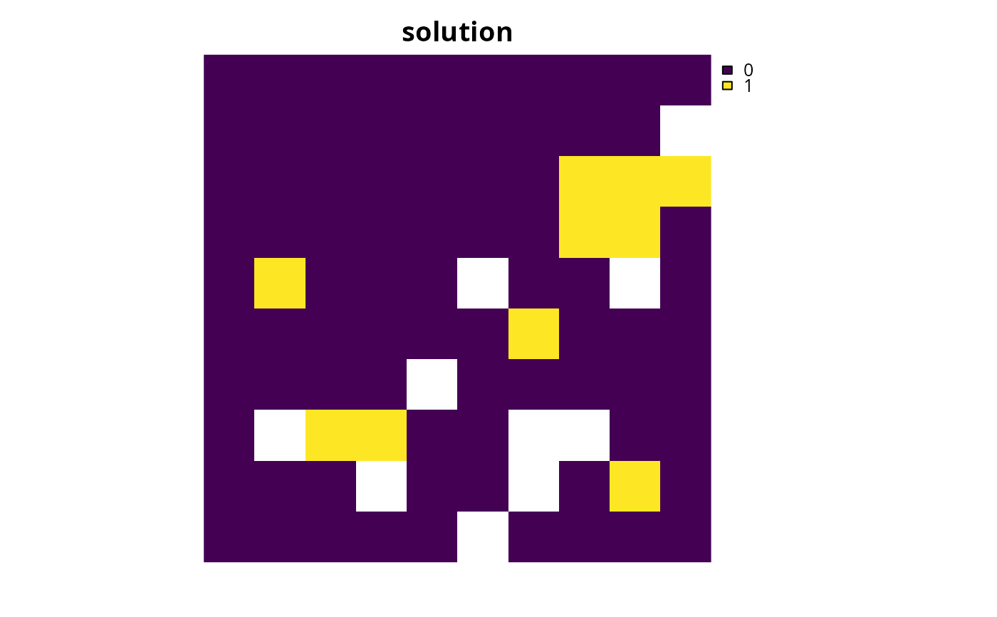
# create minimal problem to show the correct method for setting
# weights for problems with manual targets
p8 <-
  problem(sim_pu_raster, sim_features) %>%
  add_max_n_targets_met_objective(budget = 3000) %>%
  add_manual_targets(
    data.frame(
    feature = c("feature_1", "feature_4"),
    type = "relative",
    target = 0.1)
  ) %>%
  add_feature_weights(matrix(c(1, 200), ncol = 1)) %>%
  add_binary_decisions() %>%
  add_default_solver(verbose = FALSE)

# solve problem
s8 <- solve(p8)

# plot solution
plot(s8, main = "solution", axes = FALSE)