Add maximum phylogenetic diversity objective
Source:R/add_max_phylo_div_objective.R
add_max_phylo_div_objective.RdSet the objective of a conservation planning problem to
maximize the phylogenetic diversity of the features represented in the
solution subject to a budget. This objective is similar to
add_max_n_targets_met_objective() except
that emphasis is placed on representing a phylogenetically diverse set of
species, rather than as many features as possible (subject to weights).
This function was inspired by Faith (1992) and Rodrigues et al.
(2002).
Arguments
- x
problem()object.- budget
numericvalue specifying the maximum expenditure permitted for the solution. Ifxhas multiple zones, thenbudgetcan be (i) a singlenumericvalue to specify an overall budget for the entire solution or (ii) anumericvector to specify a budget for each zone (separately) in the solution.- tree
ape::phylo()object specifying a phylogenetic tree for the features inx.
Details
The maximum phylogenetic diversity objective finds the set of
planning units that meets as many representation targets for a phylogenetic
tree as possible, while staying within a fixed budget.
Note that this objective is similar to the maximum number of targets met
objective (add_max_n_targets_met_objective()) in that it
allows for both a budget and targets to be set for each feature. However,
unlike the maximum number of targets met objective, the aim of this
objective is to
maximize the total phylogenetic diversity of the targets met in the
solution, so if multiple targets are provided for a single feature, the
problem will only need to meet a single target for that feature
for the phylogenetic benefit for that feature to be counted when
calculating the phylogenetic diversity of the solution. In other words,
for multi-zone problems, this objective does not aim to maximize the
phylogenetic diversity in each zone, but rather this objective
aims to maximize the phylogenetic diversity of targets that can be met
through allocating planning units to any of the different zones in a
problem. This can be useful for problems where targets pertain to the total
amount held for each feature across multiple zones. For example,
each feature might have a non-zero amount of suitable habitat in each
planning unit when the planning units are assigned to a (i) not restored,
(ii) partially restored, or (iii) completely restored management zone.
Here each target corresponds to a single feature and can be met through
the total amount of habitat in planning units present to the three
zones.
Mathematical formulation
This objective can be expressed mathematically for a set of planning units (\(I\) indexed by \(i\)) and a set of features (\(J\) indexed by \(j\)) as:
$$\mathit{Maximize} \space \sum_{j = 1}^{J} m_b l_b \\ \mathit{subject \space to} \\ \sum_{i = 1}^{I} x_i r_{ij} \geq y_j t_j \forall j \in J \\ m_b \leq y_j \forall j \in T(b) \\ \sum_{i = 1}^{I} x_i c_i \leq B$$
Here, \(x_i\) is the decisions variable (e.g., specifying whether planning unit \(i\) has been selected (1) or not (0)), \(r_{ij}\) is the amount of feature \(j\) in planning unit \(i\), \(t_j\) is the representation target for feature \(j\), \(y_j\) indicates if the solution has meet the target \(t_j\) for feature \(j\). Additionally, \(T\) represents a phylogenetic tree containing features \(j\) and has the branches \(b\) associated within lengths \(l_b\). The binary variable \(m_b\) denotes if at least one feature associated with the branch \(b\) has met its representation as indicated by \(y_j\). For brevity, we denote the features \(j\) associated with branch \(b\) using \(T(b)\). Finally, \(B\) is the budget allocated for the solution, and \(c_i\) is the cost of planning unit \(i\).
Notes
In early versions, this function was named as the
add_max_phylo_objective() function.
Additionally, in previous versions (< 9.0.0), this function had extra
terms to help minimize the solution cost. Although these terms
have since been removed to reduce solve time,
this behavior can still be achieved by
building a multi-objective optimization problem and specifying the
first problem based on this objective function and the second
problem based on minimizing cost penalties (i.e., by using
add_min_penalties_objective() and add_cost_penalties()).
References
Faith DP (1992) Conservation evaluation and phylogenetic diversity. Biological Conservation, 61: 1–10.
Rodrigues ASL and Gaston KJ (2002) Maximising phylogenetic diversity in the selection of networks of conservation areas. Biological Conservation, 105: 103–111.
Examples
# load ape package
require(ape)
# load data
sim_pu_raster <- get_sim_pu_raster()
sim_features <- get_sim_features()
sim_phylogeny <- get_sim_phylogeny()
sim_zones_pu_raster <- get_sim_zones_pu_raster()
sim_zones_features <- get_sim_zones_features()
# plot the simulated phylogeny
par(mfrow = c(1, 1))
plot(sim_phylogeny, main = "phylogeny")
 # create problem with a maximum phylogenetic diversity objective,
# where each feature needs 10% of its distribution to be secured for
# it to be adequately conserved and a total budget of 1900
p1 <-
problem(sim_pu_raster, sim_features) %>%
add_max_phylo_div_objective(1900, sim_phylogeny) %>%
add_relative_targets(0.1) %>%
add_binary_decisions() %>%
add_default_solver(verbose = FALSE)
# solve problem
s1 <- solve(p1)
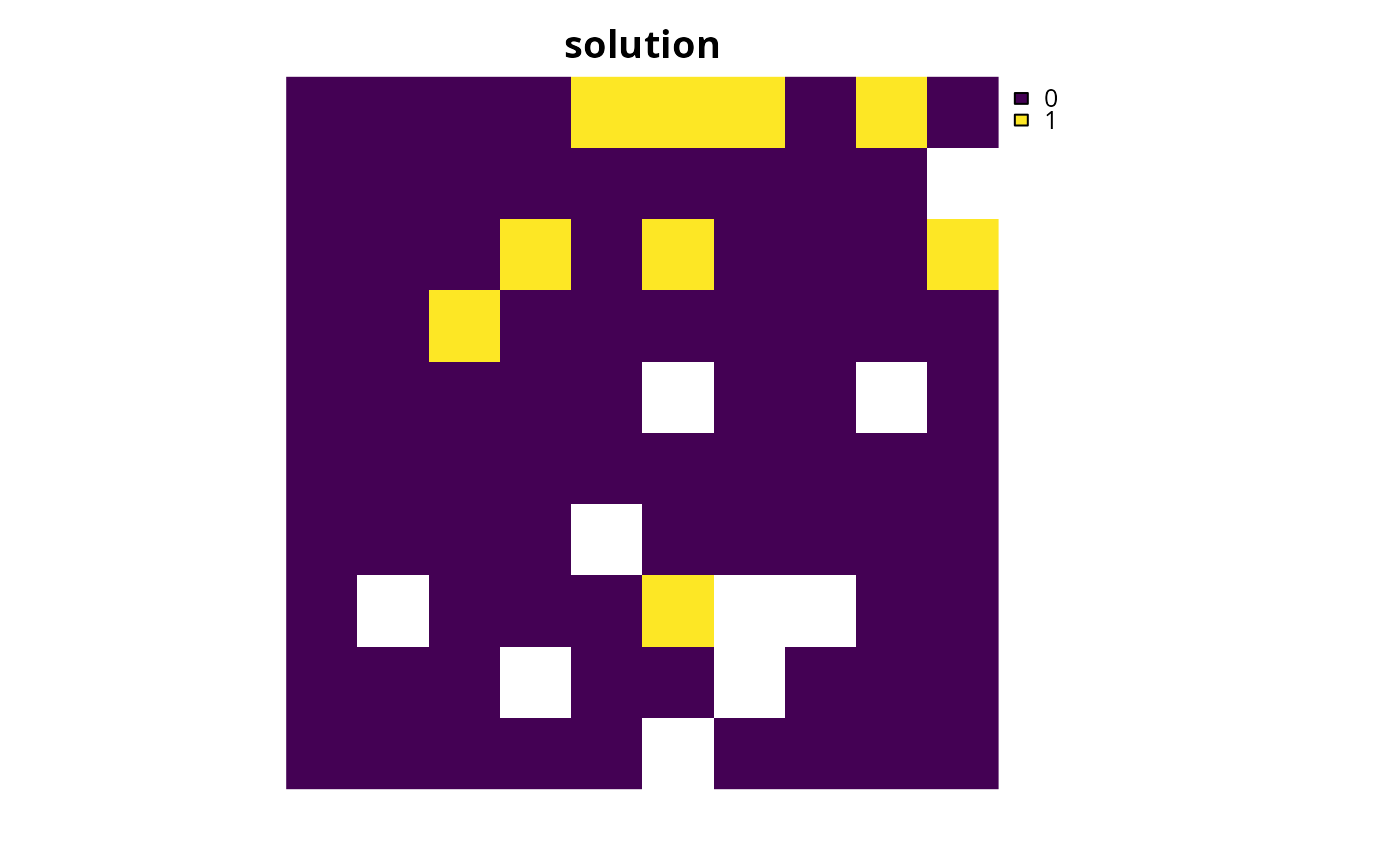
# plot solution
plot(s1, main = "solution", axes = FALSE)
# create problem with a maximum phylogenetic diversity objective,
# where each feature needs 10% of its distribution to be secured for
# it to be adequately conserved and a total budget of 1900
p1 <-
problem(sim_pu_raster, sim_features) %>%
add_max_phylo_div_objective(1900, sim_phylogeny) %>%
add_relative_targets(0.1) %>%
add_binary_decisions() %>%
add_default_solver(verbose = FALSE)
# solve problem
s1 <- solve(p1)
# plot solution
plot(s1, main = "solution", axes = FALSE)
 # find out which features have their targets met
r1 <- eval_target_coverage_summary(p1, s1)
print(r1, width = Inf)
#> # A tibble: 5 × 10
#> feature met total_amount absolute_target absolute_held absolute_shortfall
#> <chr> <lgl> <dbl> <dbl> <dbl> <dbl>
#> 1 feature_1 FALSE 83.3 8.33 6.84 1.49
#> 2 feature_2 TRUE 31.2 3.12 3.24 0
#> 3 feature_3 FALSE 72.0 7.20 6.02 1.18
#> 4 feature_4 TRUE 42.7 4.27 4.31 0
#> 5 feature_5 FALSE 56.7 5.67 4.70 0.973
#> relative_target relative_held relative_shortfall relative_met
#> <dbl> <dbl> <dbl> <dbl>
#> 1 0.1 0.0821 0.179 0.821
#> 2 0.1 0.104 0 1
#> 3 0.1 0.0836 0.164 0.836
#> 4 0.1 0.101 0 1
#> 5 0.1 0.0828 0.172 0.828
# plot the phylogeny and color the adequately represented features in red
plot(
sim_phylogeny, main = "adequately represented features",
tip.color = replace(
rep("black", terra::nlyr(sim_features)),
sim_phylogeny$tip.label %in% r1$feature[r1$met], "red"
)
)
# find out which features have their targets met
r1 <- eval_target_coverage_summary(p1, s1)
print(r1, width = Inf)
#> # A tibble: 5 × 10
#> feature met total_amount absolute_target absolute_held absolute_shortfall
#> <chr> <lgl> <dbl> <dbl> <dbl> <dbl>
#> 1 feature_1 FALSE 83.3 8.33 6.84 1.49
#> 2 feature_2 TRUE 31.2 3.12 3.24 0
#> 3 feature_3 FALSE 72.0 7.20 6.02 1.18
#> 4 feature_4 TRUE 42.7 4.27 4.31 0
#> 5 feature_5 FALSE 56.7 5.67 4.70 0.973
#> relative_target relative_held relative_shortfall relative_met
#> <dbl> <dbl> <dbl> <dbl>
#> 1 0.1 0.0821 0.179 0.821
#> 2 0.1 0.104 0 1
#> 3 0.1 0.0836 0.164 0.836
#> 4 0.1 0.101 0 1
#> 5 0.1 0.0828 0.172 0.828
# plot the phylogeny and color the adequately represented features in red
plot(
sim_phylogeny, main = "adequately represented features",
tip.color = replace(
rep("black", terra::nlyr(sim_features)),
sim_phylogeny$tip.label %in% r1$feature[r1$met], "red"
)
)
 # rename the features in the example phylogeny for use with the
# multi-zone data
sim_phylogeny$tip.label <- feature_names(sim_zones_features)
# create targets for a multi-zone problem. Here, each feature needs a total
# of 10 units of habitat to be conserved among the three zones to be
# considered adequately conserved
targets <- tibble::tibble(
feature = feature_names(sim_zones_features),
zone = list(zone_names(sim_zones_features))[
rep(1, number_of_features(sim_zones_features))],
type = rep("absolute", number_of_features(sim_zones_features)),
target = rep(10, number_of_features(sim_zones_features))
)
# create a multi-zone problem with a maximum phylogenetic diversity
# objective, where the total expenditure in all zones is 5000.
p2 <-
problem(sim_zones_pu_raster, sim_zones_features) %>%
add_max_phylo_div_objective(5000, sim_phylogeny) %>%
add_manual_targets(targets) %>%
add_binary_decisions() %>%
add_default_solver(verbose = FALSE)
# solve problem
s2 <- solve(p2)
# plot solution
plot(category_layer(s2), main = "solution", axes = FALSE)
# rename the features in the example phylogeny for use with the
# multi-zone data
sim_phylogeny$tip.label <- feature_names(sim_zones_features)
# create targets for a multi-zone problem. Here, each feature needs a total
# of 10 units of habitat to be conserved among the three zones to be
# considered adequately conserved
targets <- tibble::tibble(
feature = feature_names(sim_zones_features),
zone = list(zone_names(sim_zones_features))[
rep(1, number_of_features(sim_zones_features))],
type = rep("absolute", number_of_features(sim_zones_features)),
target = rep(10, number_of_features(sim_zones_features))
)
# create a multi-zone problem with a maximum phylogenetic diversity
# objective, where the total expenditure in all zones is 5000.
p2 <-
problem(sim_zones_pu_raster, sim_zones_features) %>%
add_max_phylo_div_objective(5000, sim_phylogeny) %>%
add_manual_targets(targets) %>%
add_binary_decisions() %>%
add_default_solver(verbose = FALSE)
# solve problem
s2 <- solve(p2)
# plot solution
plot(category_layer(s2), main = "solution", axes = FALSE)
 # find out which features have their targets met
r2 <- eval_target_coverage_summary(p2, s2)
print(r2, width = Inf)
#> # A tibble: 5 × 12
#> feature zone sense met total_amount absolute_target absolute_held
#> <chr> <list> <chr> <lgl> <dbl> <dbl> <dbl>
#> 1 feature_1 <chr [3]> >= TRUE 250. 10 19.5
#> 2 feature_2 <chr [3]> >= FALSE 93.6 10 7.17
#> 3 feature_3 <chr [3]> >= TRUE 216. 10 16.6
#> 4 feature_4 <chr [3]> >= TRUE 128. 10 10.2
#> 5 feature_5 <chr [3]> >= TRUE 170. 10 13.2
#> absolute_shortfall relative_target relative_held relative_shortfall
#> <dbl> <dbl> <dbl> <dbl>
#> 1 0 0.0400 0.0781 0
#> 2 2.83 0.107 0.0766 0.283
#> 3 0 0.0463 0.0770 0
#> 4 0 0.0781 0.0796 0
#> 5 0 0.0588 0.0776 0
#> relative_met
#> <dbl>
#> 1 1
#> 2 0.717
#> 3 1
#> 4 1
#> 5 1
# plot the phylogeny and color the adequately represented features in red
plot(
sim_phylogeny, main = "adequately represented features",
tip.color = replace(
rep("black", terra::nlyr(sim_features)), which(r2$met), "red"
)
)
# find out which features have their targets met
r2 <- eval_target_coverage_summary(p2, s2)
print(r2, width = Inf)
#> # A tibble: 5 × 12
#> feature zone sense met total_amount absolute_target absolute_held
#> <chr> <list> <chr> <lgl> <dbl> <dbl> <dbl>
#> 1 feature_1 <chr [3]> >= TRUE 250. 10 19.5
#> 2 feature_2 <chr [3]> >= FALSE 93.6 10 7.17
#> 3 feature_3 <chr [3]> >= TRUE 216. 10 16.6
#> 4 feature_4 <chr [3]> >= TRUE 128. 10 10.2
#> 5 feature_5 <chr [3]> >= TRUE 170. 10 13.2
#> absolute_shortfall relative_target relative_held relative_shortfall
#> <dbl> <dbl> <dbl> <dbl>
#> 1 0 0.0400 0.0781 0
#> 2 2.83 0.107 0.0766 0.283
#> 3 0 0.0463 0.0770 0
#> 4 0 0.0781 0.0796 0
#> 5 0 0.0588 0.0776 0
#> relative_met
#> <dbl>
#> 1 1
#> 2 0.717
#> 3 1
#> 4 1
#> 5 1
# plot the phylogeny and color the adequately represented features in red
plot(
sim_phylogeny, main = "adequately represented features",
tip.color = replace(
rep("black", terra::nlyr(sim_features)), which(r2$met), "red"
)
)
 # create a multi-zone problem with a maximum phylogenetic diversity
# objective, where each zone has a separate budget.
p3 <-
problem(sim_zones_pu_raster, sim_zones_features) %>%
add_max_phylo_div_objective(c(2500, 500, 2000), sim_phylogeny) %>%
add_manual_targets(targets) %>%
add_binary_decisions() %>%
add_default_solver(verbose = FALSE)
# solve problem
s3 <- solve(p3)
# plot solution
plot(category_layer(s3), main = "solution", axes = FALSE)
# create a multi-zone problem with a maximum phylogenetic diversity
# objective, where each zone has a separate budget.
p3 <-
problem(sim_zones_pu_raster, sim_zones_features) %>%
add_max_phylo_div_objective(c(2500, 500, 2000), sim_phylogeny) %>%
add_manual_targets(targets) %>%
add_binary_decisions() %>%
add_default_solver(verbose = FALSE)
# solve problem
s3 <- solve(p3)
# plot solution
plot(category_layer(s3), main = "solution", axes = FALSE)
 # find out which features have their targets met
r3 <- eval_target_coverage_summary(p3, s3)
print(r3, width = Inf)
#> # A tibble: 5 × 12
#> feature zone sense met total_amount absolute_target absolute_held
#> <chr> <list> <chr> <lgl> <dbl> <dbl> <dbl>
#> 1 feature_1 <chr [3]> >= TRUE 250. 10 16.4
#> 2 feature_2 <chr [3]> >= FALSE 93.6 10 7.54
#> 3 feature_3 <chr [3]> >= TRUE 216. 10 13.8
#> 4 feature_4 <chr [3]> >= TRUE 128. 10 10.4
#> 5 feature_5 <chr [3]> >= TRUE 170. 10 11.3
#> absolute_shortfall relative_target relative_held relative_shortfall
#> <dbl> <dbl> <dbl> <dbl>
#> 1 0 0.0400 0.0657 0
#> 2 2.46 0.107 0.0805 0.246
#> 3 0 0.0463 0.0639 0
#> 4 0 0.0781 0.0816 0
#> 5 0 0.0588 0.0663 0
#> relative_met
#> <dbl>
#> 1 1
#> 2 0.754
#> 3 1
#> 4 1
#> 5 1
# plot the phylogeny and color the adequately represented features in red
plot(
sim_phylogeny, main = "adequately represented features",
tip.color = replace(
rep("black", terra::nlyr(sim_features)), which(r3$met), "red"
)
)
# find out which features have their targets met
r3 <- eval_target_coverage_summary(p3, s3)
print(r3, width = Inf)
#> # A tibble: 5 × 12
#> feature zone sense met total_amount absolute_target absolute_held
#> <chr> <list> <chr> <lgl> <dbl> <dbl> <dbl>
#> 1 feature_1 <chr [3]> >= TRUE 250. 10 16.4
#> 2 feature_2 <chr [3]> >= FALSE 93.6 10 7.54
#> 3 feature_3 <chr [3]> >= TRUE 216. 10 13.8
#> 4 feature_4 <chr [3]> >= TRUE 128. 10 10.4
#> 5 feature_5 <chr [3]> >= TRUE 170. 10 11.3
#> absolute_shortfall relative_target relative_held relative_shortfall
#> <dbl> <dbl> <dbl> <dbl>
#> 1 0 0.0400 0.0657 0
#> 2 2.46 0.107 0.0805 0.246
#> 3 0 0.0463 0.0639 0
#> 4 0 0.0781 0.0816 0
#> 5 0 0.0588 0.0663 0
#> relative_met
#> <dbl>
#> 1 1
#> 2 0.754
#> 3 1
#> 4 1
#> 5 1
# plot the phylogeny and color the adequately represented features in red
plot(
sim_phylogeny, main = "adequately represented features",
tip.color = replace(
rep("black", terra::nlyr(sim_features)), which(r3$met), "red"
)
)
