Add maximum utility objective

Set the objective of a conservation planning problem to maximize the weighted sum of the features represented by the solution as much as possible without exceeding a budget. This objective does not use targets, and feature weights should be used instead to increase the representation of particular features by a solution. Note that this objective does not aim to maximize as much of each feature individually, and so often results in solutions that are heavily biased towards just a few features.

Usage

add_max_utility_objective(x, budget)

Arguments

x: problem() object.
budget: numeric value specifying the maximum expenditure of the prioritization. For problems with multiple zones, the argument to budget can be (i) a single numeric value to specify a single budget for the entire solution or (ii) a numeric vector to specify a separate budget for each management zone.

Value

An updated problem() object with the objective added to it.

Details

The maximum utility objective seeks to maximize the overall level of representation across a suite of conservation features, while keeping cost within a fixed budget. Additionally, weights can be used to favor the representation of particular features over other features (see add_feature_weights()). It is essentially calculated as a weighted sum of the feature data inside the selected planning units.

Mathematical formulation

This objective can be expressed mathematically for a set of planning units ($I$ indexed by $i$) and a set of features ($J$ indexed by $j$) as:

$$\mathit{Maximize} \space \sum_{i = 1}^{I} -s \space c_i \space x_i + \sum_{j = 1}^{J} a_j w_j \\ \mathit{subject \space to} \\ a_j = \sum_{i = 1}^{I} x_i r_{ij} \space \forall j \in J \\ \sum_{i = 1}^{I} x_i c_i \leq B$$

Here, $x_i$ is the decisions variable (e.g., specifying whether planning unit $i$ has been selected (1) or not (0)), $r_{ij}$ is the amount of feature $j$ in planning unit $i$, $a_j$ is the amount of feature $j$ represented in in the solution, and $w_j$ is the weight for feature $j$ (defaults to 1 for all features; see add_feature_weights() to specify weights). Additionally, $B$ is the budget allocated for the solution, $c_i$ is the cost of planning unit $i$, and $s$ is a scaling factor used to shrink the costs so that the problem will return a cheapest solution when there are multiple solutions that represent the same amount of all features within the budget.

Notes

In early versions (< 3.0.0.0), this function was named as the add_max_cover_objective function. It was renamed to avoid confusion with existing terminology.

Examples

# \dontrun{
# load data
sim_pu_raster <- get_sim_pu_raster()
sim_features <- get_sim_features()
sim_zones_pu_raster <- get_sim_zones_pu_raster()
sim_zones_features <- get_sim_zones_features()

# create problem with maximum utility objective
p1 <-
  problem(sim_pu_raster, sim_features) %>%
  add_max_utility_objective(5000) %>%
  add_binary_decisions() %>%
  add_default_solver(gap = 0, verbose = FALSE)

# solve problem
s1 <- solve(p1)

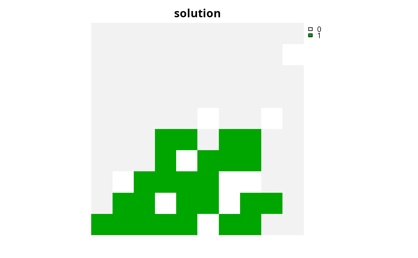
# plot solution
plot(s1, main = "solution", axes = FALSE)


# create multi-zone problem with maximum utility objective that
# has a single budget for all zones
p2 <-
  problem(sim_zones_pu_raster, sim_zones_features) %>%
  add_max_utility_objective(5000) %>%
  add_binary_decisions() %>%
  add_default_solver(gap = 0, verbose = FALSE)

# solve problem
s2 <- solve(p2)

# plot solution
plot(category_layer(s2), main = "solution", axes = FALSE)


# create multi-zone problem with maximum utility objective that
# has separate budgets for each zone
p3 <-
  problem(sim_zones_pu_raster, sim_zones_features) %>%
  add_max_utility_objective(c(1000, 2000, 3000)) %>%
  add_binary_decisions() %>%
  add_default_solver(gap = 0, verbose = FALSE)

# solve problem
s3 <- solve(p3)

# plot solution
plot(category_layer(s3), main = "solution", axes = FALSE)

# }