Add maximum feature representation objective

Set the objective of a conservation planning problem to fulfill as many targets as possible, whilst ensuring that the cost of the solution does not exceed a budget.

Usage

add_max_features_objective(x, budget)

Arguments

x: problem() object.
budget: numeric value specifying the maximum expenditure of the prioritization. For problems with multiple zones, the argument to budget can be (i) a single numeric value to specify a single budget for the entire solution or (ii) a numeric vector to specify a separate budget for each management zone.

Value

An updated problem() object with the objective added to it.

Details

The maximum feature representation objective is an enhanced version of the maximum coverage objective add_max_cover_objective() because targets can be used to ensure that a certain amount of each feature is required in order for them to be adequately represented (similar to the minimum set objective (see add_min_set_objective()). This objective finds the set of planning units that meets representation targets for as many features as possible while staying within a fixed budget (inspired by Cabeza and Moilanen 2001). Additionally, weights can be used add_feature_weights()). If multiple solutions can meet the same number of weighted targets while staying within budget, the cheapest solution is returned.

Mathematical formulation

This objective can be expressed mathematically for a set of planning units ($I$ indexed by $i$) and a set of features ($J$ indexed by $j$) as:

$$\mathit{Maximize} \space \sum_{i = 1}^{I} -s \space c_i \space x_i + \sum_{j = 1}^{J} y_j w_j \\ \mathit{subject \space to} \\ \sum_{i = 1}^{I} x_i r_{ij} \geq y_j t_j \forall j \in J \\ \sum_{i = 1}^{I} x_i c_i \leq B$$

Here, $x_i$ is the decisions variable (e.g., specifying whether planning unit $i$ has been selected (1) or not (0)), $r_{ij}$ is the amount of feature $j$ in planning unit $i$, $t_j$ is the representation target for feature $j$, $y_j$ indicates if the solution has meet the target $t_j$ for feature $j$, and $w_j$ is the weight for feature $j$ (defaults to 1 for all features; see add_feature_weights() to specify weights). Additionally, $B$ is the budget allocated for the solution, $c_i$ is the cost of planning unit $i$, and $s$ is a scaling factor used to shrink the costs so that the problem will return a cheapest solution when there are multiple solutions that represent the same amount of all features within the budget.

References

Cabeza M and Moilanen A (2001) Design of reserve networks and the persistence of biodiversity. Trends in Ecology & Evolution, 16: 242--248.

Examples

# \dontrun{
# load data
sim_pu_raster <- get_sim_pu_raster()
sim_features <- get_sim_features()
sim_zones_pu_raster <- get_sim_zones_pu_raster()
sim_zones_features <- get_sim_zones_features()

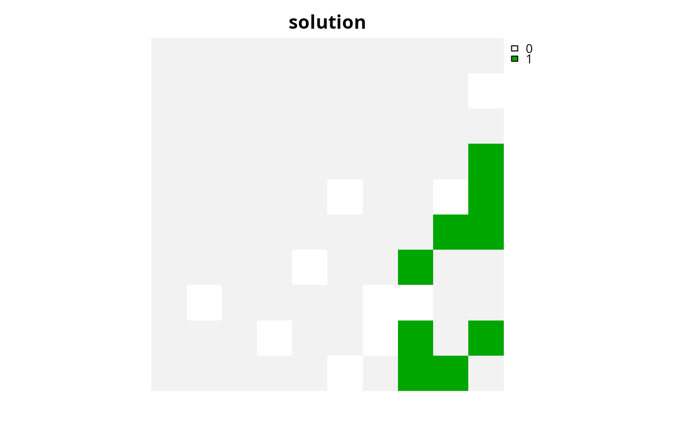
# create problem with maximum features objective
p1 <-
  problem(sim_pu_raster, sim_features) %>%
  add_max_features_objective(1800) %>%
  add_relative_targets(0.1) %>%
  add_binary_decisions() %>%
  add_default_solver(verbose = FALSE)

# solve problem
s1 <- solve(p1)

# plot solution
plot(s1, main = "solution", axes = FALSE)


# create multi-zone problem with maximum features objective,
# with 10% representation targets for each feature, and set
# a budget such that the total maximum expenditure in all zones
# cannot exceed 3000
p2 <-
  problem(sim_zones_pu_raster, sim_zones_features) %>%
  add_max_features_objective(3000) %>%
  add_relative_targets(matrix(0.1, ncol = 3, nrow = 5)) %>%
  add_binary_decisions() %>%
  add_default_solver(verbose = FALSE)

# solve problem
s2 <- solve(p2)

# plot solution
plot(category_layer(s2), main = "solution", axes = FALSE)


# create multi-zone problem with maximum features objective,
# with 10% representation targets for each feature, and set
# separate budgets for each management zone
p3 <-
  problem(sim_zones_pu_raster, sim_zones_features) %>%
  add_max_features_objective(c(3000, 3000, 3000)) %>%
  add_relative_targets(matrix(0.1, ncol = 3, nrow = 5)) %>%
  add_binary_decisions() %>%
  add_default_solver(verbose = FALSE)

# solve problem
s3 <- solve(p3)

# plot solution
plot(category_layer(s3), main = "solution", axes = FALSE)

# }