Add maximum coverage objective

Set the objective of a conservation planning problem to represent at least one instance of as many features as possible within a given budget. This objective does not use targets, and feature weights should be used instead to increase the representation of certain features by a solution.

Usage

add_max_cover_objective(x, budget)

Arguments

x: problem() object.
budget: numeric value specifying the maximum expenditure of the prioritization. For problems with multiple zones, the argument to budget can be a single numeric value to specify a budget for the entire solution or a numeric vector to specify a budget for each each management zone.

Value

An updated problem() object with the objective added to it.

Details

The maximum coverage objective seeks to find the set of planning units that maximizes the number of represented features, while keeping cost within a fixed budget. Here, features are treated as being represented if the reserve system contains at least a single instance of a feature (i.e., an amount greater than 1). This formulation has often been used in conservation planning problems dealing with binary biodiversity data that indicate the presence/absence of suitable habitat (e.g., Church & Velle 1974). Additionally, weights can be used to favor the representation of certain features over other features (see add_feature_weights()). Check out the add_max_features_objective() for a more generalized formulation which can accommodate user-specified representation targets.

Mathematical formulation

This objective is based on the maximum coverage reserve selection problem (Church & Velle 1974; Church et al. 1996). The maximum coverage objective for the reserve design problem can be expressed mathematically for a set of planning units ($I$ indexed by $i$) and a set of features ($J$ indexed by $j$) as:

$$\mathit{Maximize} \space \sum_{i = 1}^{I} -s \space c_i \space x_i + \sum_{j = 1}^{J} y_j w_j \\ \mathit{subject \space to} \\ \sum_{i = 1}^{I} x_i r_{ij} \geq y_j \times 1 \forall j \in J \\ \sum_{i = 1}^{I} x_i c_i \leq B$$

Here, $x_i$ is the decisions variable (e.g., specifying whether planning unit $i$ has been selected (1) or not (0)), $r_{ij}$ is the amount of feature $j$ in planning unit $i$, $y_j$ indicates if the solution has meet the target $t_j$ for feature $j$, and $w_j$ is the weight for feature $j$ (defaults to 1 for all features; see add_feature_weights() to specify weights). Additionally, $B$ is the budget allocated for the solution, $c_i$ is the cost of planning unit $i$, and $s$ is a scaling factor used to shrink the costs so that the problem will return a cheapest solution when there are multiple solutions that represent the same amount of all features within the budget.

Notes

In early versions (< 3.0.0.0), the mathematical formulation underpinning this function was very different. Specifically, as described above, the function now follows the formulations outlined in Church et al. (1996). The old formulation is now provided by the add_max_utility_objective() function.

References

Church RL and Velle CR (1974) The maximum covering location problem. Regional Science, 32: 101--118.

Church RL, Stoms DM, and Davis FW (1996) Reserve selection as a maximum covering location problem. Biological Conservation, 76: 105--112.

Examples

# \dontrun{
# load data
sim_pu_raster <- get_sim_pu_raster()
sim_zones_pu_raster <- get_sim_zones_pu_raster()
sim_features <- get_sim_features()
sim_zones_features <- get_sim_zones_features()

# threshold the feature data to generate binary biodiversity data
sim_binary_features <- sim_features
thresholds <- terra::global(
  sim_features, fun = quantile, probs = 0.5, na.rm = TRUE
)
for (i in seq_len(terra::nlyr(sim_features))) {
  sim_binary_features[[i]] <- terra::as.int(
    sim_features[[i]] > thresholds[[1]][[i]]
  )
}

# create problem with maximum cover objective
p1 <-
  problem(sim_pu_raster, sim_binary_features) %>%
  add_max_cover_objective(500) %>%
  add_binary_decisions() %>%
  add_default_solver(verbose = FALSE)

# solve problem
s1 <- solve(p1)

# plot solution
plot(s1, main = "solution", axes = FALSE)


# threshold the multi-zone feature data to generate binary biodiversity data
sim_binary_features_zones <- sim_zones_features
for (z in seq_len(number_of_zones(sim_zones_features))) {
  thresholds <- terra::global(
    sim_zones_features[[z]], fun = quantile, probs = 0.5, na.rm = TRUE
  )
  for (i in seq_len(number_of_features(sim_zones_features))) {
    sim_binary_features_zones[[z]][[i]] <- terra::as.int(
      sim_zones_features[[z]][[i]] > thresholds[[1]][[i]]
    )
  }
}

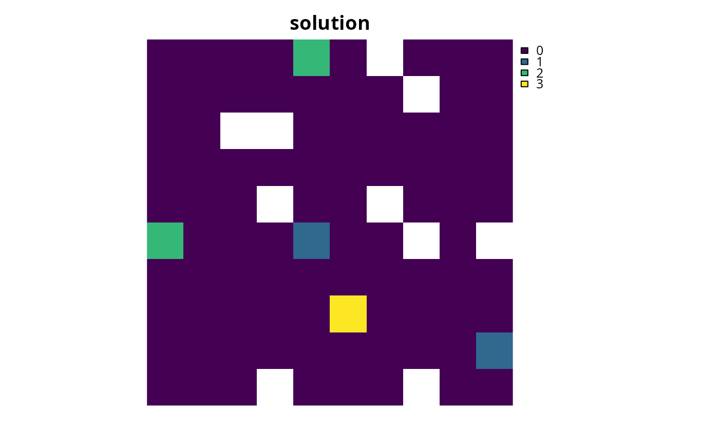
# create multi-zone problem with maximum cover objective that
# has a single budget for all zones
p2 <-
  problem(sim_zones_pu_raster, sim_binary_features_zones) %>%
  add_max_cover_objective(800) %>%
  add_binary_decisions() %>%
  add_default_solver(verbose = FALSE)

# solve problem
s2 <- solve(p2)

# plot solution
plot(category_layer(s2), main = "solution", axes = FALSE)


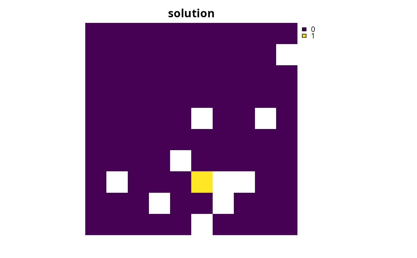
# create multi-zone problem with maximum cover objective that
# has separate budgets for each zone
p3 <-
  problem(sim_zones_pu_raster, sim_binary_features_zones) %>%
  add_max_cover_objective(c(400, 400, 400)) %>%
  add_binary_decisions() %>%
  add_default_solver(verbose = FALSE)

# solve problem
s3 <- solve(p3)

# plot solution
plot(category_layer(s3), main = "solution", axes = FALSE)

# }