Evaluate target coverage by solution
Source:R/eval_target_coverage_summary.R
eval_target_coverage_summary.RdCalculate how well feature representation targets are met by a solution to a conservation planning problem. It is useful for understanding if features are adequately represented by a solution. Note that this function can only be used with problems that contain targets.
Usage
eval_target_coverage_summary(
  x,
  solution,
  include_zone = number_of_zones(x) > 1,
  include_sense = number_of_zones(x) > 1
)

# S3 method for class 'ConservationProblem'
eval_target_coverage_summary(
  x,
  solution,
  include_zone = number_of_zones(x) > 1,
  include_sense = number_of_zones(x) > 1
)

# S3 method for class 'MultiConservationProblem'
eval_target_coverage_summary(
  x,
  solution,
  include_zone = number_of_zones(x) > 1,
  include_sense = number_of_zones(x) > 1
)
Arguments
- x
problem()ormulti_problem()object.- solution
numeric,matrix,data.frame,terra::rast(), orsf::sf()object. Note thatsolutionmust have the same format as the planning unit data inx. See the Solution format section for more information.- include_zone
logicalvalue indicating if the returned object should contain azonecolumn? Defaults toTRUEifxhas multiple zones.- include_sense
logicalvalue indicating if the returned object should contain asensecolumn? Defaults toTRUEifxhas multiple zones.
Value
A tibble::tibble() object.
Here, each row provides information for a different target.
It contains the following columns.
- problem
charactername of problem. Note that this column is only present ifxis amulti_problem()object.- feature
charactername of the feature associated with each target.- zone
listofcharacterzone names associated with each target. This column is in a list-column format because a single target can correspond to multiple zones (seeadd_manual_targets()for details and examples). For an example of converting the list-column format to a standardcharactercolumn format, please see the Examples section. This column is only included ifinclude_zones = TRUE.- sense
charactersense associated with each target. Sense values specify the nature of the target. Typically (e.g., when using theadd_absolute_targets()oradd_relative_targets()functions), targets are specified using sense values indicating that the total amount of a feature held within a solution (ideally) be greater than or equal to a threshold amount (i.e., a sense value of">="). Additionally, targets (i.e., using theadd_manual_targets()function) can also be specified using sense values indicating that the total amount of a feature held within a solution must be equal to a threshold amount (i.e., a sense value of"=") or smaller than or equal to a threshold amount (i.e., a sense value of"<="). This column is only included ifinclude_sense = TRUE.- met
logicalindicating if each target is met by the solution. This column is calculated by checking if the total shortfall associated with each target (i.e.,"absolute_shortfall" column) is equal to zero.- total_amount
numerictotal amount of the feature available across the entire conservation planning problem for meeting each target (not just planning units selected within the solution). Ifxhas a single zone, then this column is calculated as the sum of all of the values for a given feature (similar to values in thetotal_amountcolumn produced by theeval_feature_representation_summary()function). Otherwise, ifxhas multiple zones, then this column is calculated as the sum of the values for the feature associated with target (per the"feature"column), across the zones associated with the target (per the"zone"column).- absolute_target
numerictotal threshold amount associated with each target.- absolute_held
numerictotal amount held within the solution for the feature and (if relevant) zones associated with each target (per the"feature"and"zone"columns, respectively). This column is calculated as the sum of the feature data, supplied when creating aproblem()object (e.g., presence/absence values), weighted by the status of each planning unit in the solution (e.g., selected or not for prioritization).- absolute_shortfall
numerictotal amount by which the solution fails to meet each target. This column is calculated as the difference between the total amount held within the solution for the feature and (if relevant) zones associated with the target (i.e.,"absolute_held"column) and the target total threshold amount (i.e.,"absolute_target"column), with values set to zero depending on the sense specified for the target (e.g., if the target sense is>=then the difference is set to zero if the value in the"absolute_held"is smaller than that in the"absolute_target"column).- relative_target
numericproportion threshold amount associated with each target. This column is calculated by dividing the total threshold amount associated with each target (i.e.,"absolute_target"column) by the total amount associated with each target (i.e.,"total_amount"column).- relative_held
numericproportion held within the solution for the feature and (if relevant) zones associated with each target (per the"feature"and"zone"columns, respectively). This column is calculated by dividing the total amount held for each target (i.e.,"absolute_held"column) by the total amount for with each target (i.e.,"total_amount"column). Since this metric is only appropriate for describing how well a solution meets targets that have a">="sense, targets with a"<="or"="sense are assigned missing (NA) values in this column.- relative_shortfall
numericproportion by which the solution fails to meet each target. This column is calculated by dividing the total shortfall for each target (i.e.,"absolute_shortfall"column) by the total threshold amount associated with each target (i.e.,"absolute_target"column).- relative_met
numericproportion of the target that is fulfilled by the solution. This column is calculated by expressing the amount held by the solution (i.e.,"absolute_held"column) as a fraction of the target threshold. Since this metric is only appropriate for describing how well a solution meets targets that have a">="sense, targets with a"<="or"="sense are assigned missing (NA) values in this column.
Notes
In prior versions (< 8.0.6.7), this function calculated the
relative shortfall for a target by dividing the total shortfall for
the target (i.e., "absolute_shortfall" column) by the
total amount associated with each target (i.e.,
"total_amount" column). This was subsequently changed to ensure
consistency with the minimum shortfall objective
(add_min_shortfall_objective()).
Solution format
Broadly speaking, solution must be in the same format as
the planning unit data in x.
Further details on the correct format are listed separately
for each of the different planning unit data formats.
xhasnumericplanning unitsHere
solutionmust be anumericvector with each element corresponding to a different planning unit. It should have the same number of planning units as those inx. Additionally, any planning units with missing cost (NA) values should also have missing (NA) values in thesolution.xhasmatrixplanning unitsHere
solutionmust be amatrixvector with each row corresponding to a different planning unit, and each column correspond to a different management zone. It should have the same number of planning units and zones as those inx. Additionally, any planning units with missing cost (NA) values for a particular zone should also have a missing (NA) values insolution.xhasterra::rast()planning unitsHere
solutionbe aterra::rast()object where different cells correspond to different planning units and layers correspond to a different management zones. It should have the same dimensionality (rows, columns, layers), resolution, extent, and coordinate reference system as the planning units inx. Additionally, any planning units with missing cost (NA) values for a particular zone should also have missing (NA) values insolution.xhasdata.frameplanning unitsHere
solutionmust be adata.framewith each column corresponding to a different zone, each row corresponding to a different planning unit, and cell values corresponding to the solution value. This means that if adata.frameobject containing the solution also contains additional columns, then these columns will need to be subsetted prior to using this function (see below for example withsf::sf()data). Additionally, any planning units with missing cost (NA) values for a particular zone should also have missing (NA) values insolution.xhassf::sf()planning unitsHere
solutionmust be asf::sf()object with each column corresponding to a different zone, each row corresponding to a different planning unit, and cell values corresponding to the solution value. This means that if thesf::sf()object containing the solution also contains additional columns, then these columns will need to be subsetted prior to using this function (see below for example). Additionally,solutionmust also have the same coordinate reference system as the planning unit data. Furthermore, any planning units with missing cost (NA) values for a particular zone should also have missing (NA) values insolution.
See also
See summaries for an overview of all functions for summarizing solutions.
Other functions for summarizing solutions:
eval_asym_connectivity_summary(),
eval_boundary_summary(),
eval_connectivity_summary(),
eval_cost_summary(),
eval_feature_representation_summary(),
eval_n_summary(),
eval_objective_summary()
Examples
# set seed for reproducibility
set.seed(500)
# load data
sim_pu_raster <- get_sim_pu_raster()
sim_pu_polygons <- get_sim_pu_polygons()
sim_features <- get_sim_features()
sim_zones_pu_polygons <- get_sim_zones_pu_polygons()
sim_zones_features <- get_sim_zones_features()
# build minimal conservation problem with raster data
p1 <-
problem(sim_pu_raster, sim_features) %>%
add_min_set_objective() %>%
add_relative_targets(0.1) %>%
add_binary_decisions() %>%
add_default_solver(verbose = FALSE)
# solve the problem
s1 <- solve(p1)
# print solution
print(s1)
#> class : SpatRaster
#> size : 10, 10, 1 (nrow, ncol, nlyr)
#> resolution : 0.1, 0.1 (x, y)
#> extent : 0, 1, 0, 1 (xmin, xmax, ymin, ymax)
#> coord. ref. : WGS 84 / Pseudo-Mercator (EPSG:3857)
#> source(s) : memory
#> varname : sim_pu_raster
#> name : layer
#> min value : 0
#> max value : 1
# plot solution
plot(s1, main = "solution", axes = FALSE)
 # calculate target coverage by the solution
r1 <- eval_target_coverage_summary(p1, s1)
print(r1, width = Inf) # note: `width = Inf` tells R to print all columns
#> # A tibble: 5 × 10
#> feature met total_amount absolute_target absolute_held absolute_shortfall
#> <chr> <lgl> <dbl> <dbl> <dbl> <dbl>
#> 1 feature_1 TRUE 83.3 8.33 8.91 0
#> 2 feature_2 TRUE 31.2 3.12 3.13 0
#> 3 feature_3 TRUE 72.0 7.20 7.34 0
#> 4 feature_4 TRUE 42.7 4.27 4.35 0
#> 5 feature_5 TRUE 56.7 5.67 6.01 0
#> relative_target relative_held relative_shortfall relative_met
#> <dbl> <dbl> <dbl> <dbl>
#> 1 0.1 0.107 0 1
#> 2 0.1 0.100 0 1
#> 3 0.1 0.102 0 1
#> 4 0.1 0.102 0 1
#> 5 0.1 0.106 0 1
# build minimal conservation problem with polygon data
p2 <-
problem(sim_pu_polygons, sim_features, cost_column = "cost") %>%
add_min_set_objective() %>%
add_relative_targets(0.1) %>%
add_binary_decisions() %>%
add_default_solver(verbose = FALSE)
# solve the problem
s2 <- solve(p2)
# print first six rows of the attribute table
print(head(s2))
#> Simple feature collection with 6 features and 4 fields
#> Geometry type: POLYGON
#> Dimension: XY
#> Bounding box: xmin: 0 ymin: 0.9 xmax: 0.6 ymax: 1
#> Projected CRS: WGS 84 / Pseudo-Mercator
#> # A tibble: 6 × 5
#> cost locked_in locked_out solution_1 geometry
#> <dbl> <lgl> <lgl> <dbl> <POLYGON [m]>
#> 1 216. FALSE FALSE 0 ((0 1, 0.1 1, 0.1 0.9, 0 0.9, 0 1))
#> 2 213. FALSE FALSE 0 ((0.1 1, 0.2 1, 0.2 0.9, 0.1 0.9, 0.1 1…
#> 3 207. FALSE FALSE 0 ((0.2 1, 0.3 1, 0.3 0.9, 0.2 0.9, 0.2 1…
#> 4 209. FALSE TRUE 0 ((0.3 1, 0.4 1, 0.4 0.9, 0.3 0.9, 0.3 1…
#> 5 214. FALSE FALSE 0 ((0.4 1, 0.5 1, 0.5 0.9, 0.4 0.9, 0.4 1…
#> 6 214. FALSE FALSE 0 ((0.5 1, 0.6 1, 0.6 0.9, 0.5 0.9, 0.5 1…
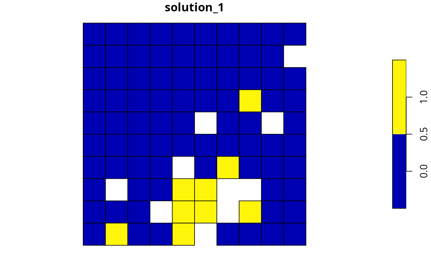
# plot solution
plot(s2[, "solution_1"])
# calculate target coverage by the solution
r1 <- eval_target_coverage_summary(p1, s1)
print(r1, width = Inf) # note: `width = Inf` tells R to print all columns
#> # A tibble: 5 × 10
#> feature met total_amount absolute_target absolute_held absolute_shortfall
#> <chr> <lgl> <dbl> <dbl> <dbl> <dbl>
#> 1 feature_1 TRUE 83.3 8.33 8.91 0
#> 2 feature_2 TRUE 31.2 3.12 3.13 0
#> 3 feature_3 TRUE 72.0 7.20 7.34 0
#> 4 feature_4 TRUE 42.7 4.27 4.35 0
#> 5 feature_5 TRUE 56.7 5.67 6.01 0
#> relative_target relative_held relative_shortfall relative_met
#> <dbl> <dbl> <dbl> <dbl>
#> 1 0.1 0.107 0 1
#> 2 0.1 0.100 0 1
#> 3 0.1 0.102 0 1
#> 4 0.1 0.102 0 1
#> 5 0.1 0.106 0 1
# build minimal conservation problem with polygon data
p2 <-
problem(sim_pu_polygons, sim_features, cost_column = "cost") %>%
add_min_set_objective() %>%
add_relative_targets(0.1) %>%
add_binary_decisions() %>%
add_default_solver(verbose = FALSE)
# solve the problem
s2 <- solve(p2)
# print first six rows of the attribute table
print(head(s2))
#> Simple feature collection with 6 features and 4 fields
#> Geometry type: POLYGON
#> Dimension: XY
#> Bounding box: xmin: 0 ymin: 0.9 xmax: 0.6 ymax: 1
#> Projected CRS: WGS 84 / Pseudo-Mercator
#> # A tibble: 6 × 5
#> cost locked_in locked_out solution_1 geometry
#> <dbl> <lgl> <lgl> <dbl> <POLYGON [m]>
#> 1 216. FALSE FALSE 0 ((0 1, 0.1 1, 0.1 0.9, 0 0.9, 0 1))
#> 2 213. FALSE FALSE 0 ((0.1 1, 0.2 1, 0.2 0.9, 0.1 0.9, 0.1 1…
#> 3 207. FALSE FALSE 0 ((0.2 1, 0.3 1, 0.3 0.9, 0.2 0.9, 0.2 1…
#> 4 209. FALSE TRUE 0 ((0.3 1, 0.4 1, 0.4 0.9, 0.3 0.9, 0.3 1…
#> 5 214. FALSE FALSE 0 ((0.4 1, 0.5 1, 0.5 0.9, 0.4 0.9, 0.4 1…
#> 6 214. FALSE FALSE 0 ((0.5 1, 0.6 1, 0.6 0.9, 0.5 0.9, 0.5 1…
# plot solution
plot(s2[, "solution_1"])
 # calculate target coverage by the solution
r2 <- eval_target_coverage_summary(p2, s2[, "solution_1"])
print(r2, width = Inf)
#> # A tibble: 5 × 10
#> feature met total_amount absolute_target absolute_held absolute_shortfall
#> <chr> <lgl> <dbl> <dbl> <dbl> <dbl>
#> 1 feature_1 TRUE 74.5 7.45 8.05 0
#> 2 feature_2 TRUE 28.1 2.81 2.83 0
#> 3 feature_3 TRUE 64.9 6.49 6.65 0
#> 4 feature_4 TRUE 38.2 3.82 3.87 0
#> 5 feature_5 TRUE 50.7 5.07 5.41 0
#> relative_target relative_held relative_shortfall relative_met
#> <dbl> <dbl> <dbl> <dbl>
#> 1 0.1 0.108 0 1
#> 2 0.1 0.101 0 1
#> 3 0.1 0.103 0 1
#> 4 0.1 0.101 0 1
#> 5 0.1 0.107 0 1
# build multi-zone conservation problem with polygon data
p3 <-
problem(
sim_zones_pu_polygons, sim_zones_features,
cost_column = c("cost_1", "cost_2", "cost_3")
) %>%
add_min_set_objective() %>%
add_relative_targets(matrix(runif(15, 0.1, 0.2), nrow = 5, ncol = 3)) %>%
add_binary_decisions() %>%
add_default_solver(verbose = FALSE)
# solve the problem
s3 <- solve(p3)
# print solution
print(s3)
#> Simple feature collection with 90 features and 9 fields
#> Geometry type: POLYGON
#> Dimension: XY
#> Bounding box: xmin: 0 ymin: 0 xmax: 1 ymax: 1
#> Projected CRS: WGS 84 / Pseudo-Mercator
#> # A tibble: 90 × 10
#> cost_1 cost_2 cost_3 locked_1 locked_2 locked_3 solution_1_zone_1
#> * <dbl> <dbl> <dbl> <lgl> <lgl> <lgl> <dbl>
#> 1 216. 183. 205. FALSE FALSE FALSE 0
#> 2 213. 189. 210. FALSE FALSE FALSE 0
#> 3 207. 194. 215. TRUE FALSE FALSE 0
#> 4 209. 198. 219. FALSE FALSE FALSE 0
#> 5 214. 200. 221. FALSE FALSE FALSE 0
#> 6 214. 203. 225. FALSE FALSE FALSE 0
#> 7 211. 209. 223. FALSE FALSE FALSE 0
#> 8 210. 212. 222. TRUE FALSE FALSE 0
#> 9 204. 218. 214. FALSE FALSE FALSE 0
#> 10 213. 183. 206. FALSE FALSE FALSE 0
#> # ℹ 80 more rows
#> # ℹ 3 more variables: solution_1_zone_2 <dbl>, solution_1_zone_3 <dbl>,
#> # geometry <POLYGON [m]>
# create new column representing the zone id that each planning unit
# was allocated to in the solution
s3$solution <- category_vector(
s3[, c("solution_1_zone_1", "solution_1_zone_2", "solution_1_zone_3")]
)
s3$solution <- factor(s3$solution)
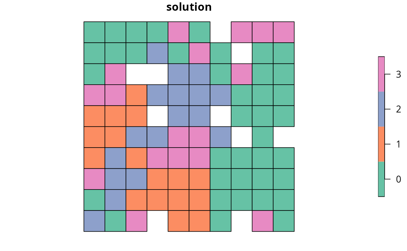
# plot solution
plot(s3[, "solution"])
# calculate target coverage by the solution
r2 <- eval_target_coverage_summary(p2, s2[, "solution_1"])
print(r2, width = Inf)
#> # A tibble: 5 × 10
#> feature met total_amount absolute_target absolute_held absolute_shortfall
#> <chr> <lgl> <dbl> <dbl> <dbl> <dbl>
#> 1 feature_1 TRUE 74.5 7.45 8.05 0
#> 2 feature_2 TRUE 28.1 2.81 2.83 0
#> 3 feature_3 TRUE 64.9 6.49 6.65 0
#> 4 feature_4 TRUE 38.2 3.82 3.87 0
#> 5 feature_5 TRUE 50.7 5.07 5.41 0
#> relative_target relative_held relative_shortfall relative_met
#> <dbl> <dbl> <dbl> <dbl>
#> 1 0.1 0.108 0 1
#> 2 0.1 0.101 0 1
#> 3 0.1 0.103 0 1
#> 4 0.1 0.101 0 1
#> 5 0.1 0.107 0 1
# build multi-zone conservation problem with polygon data
p3 <-
problem(
sim_zones_pu_polygons, sim_zones_features,
cost_column = c("cost_1", "cost_2", "cost_3")
) %>%
add_min_set_objective() %>%
add_relative_targets(matrix(runif(15, 0.1, 0.2), nrow = 5, ncol = 3)) %>%
add_binary_decisions() %>%
add_default_solver(verbose = FALSE)
# solve the problem
s3 <- solve(p3)
# print solution
print(s3)
#> Simple feature collection with 90 features and 9 fields
#> Geometry type: POLYGON
#> Dimension: XY
#> Bounding box: xmin: 0 ymin: 0 xmax: 1 ymax: 1
#> Projected CRS: WGS 84 / Pseudo-Mercator
#> # A tibble: 90 × 10
#> cost_1 cost_2 cost_3 locked_1 locked_2 locked_3 solution_1_zone_1
#> * <dbl> <dbl> <dbl> <lgl> <lgl> <lgl> <dbl>
#> 1 216. 183. 205. FALSE FALSE FALSE 0
#> 2 213. 189. 210. FALSE FALSE FALSE 0
#> 3 207. 194. 215. TRUE FALSE FALSE 0
#> 4 209. 198. 219. FALSE FALSE FALSE 0
#> 5 214. 200. 221. FALSE FALSE FALSE 0
#> 6 214. 203. 225. FALSE FALSE FALSE 0
#> 7 211. 209. 223. FALSE FALSE FALSE 0
#> 8 210. 212. 222. TRUE FALSE FALSE 0
#> 9 204. 218. 214. FALSE FALSE FALSE 0
#> 10 213. 183. 206. FALSE FALSE FALSE 0
#> # ℹ 80 more rows
#> # ℹ 3 more variables: solution_1_zone_2 <dbl>, solution_1_zone_3 <dbl>,
#> # geometry <POLYGON [m]>
# create new column representing the zone id that each planning unit
# was allocated to in the solution
s3$solution <- category_vector(
s3[, c("solution_1_zone_1", "solution_1_zone_2", "solution_1_zone_3")]
)
s3$solution <- factor(s3$solution)
# plot solution
plot(s3[, "solution"])
 # calculate target coverage by the solution
r3 <- eval_target_coverage_summary(
p3, s3[, c("solution_1_zone_1", "solution_1_zone_2", "solution_1_zone_3")]
)
print(r3, width = Inf)
#> # A tibble: 15 × 12
#> feature zone sense met total_amount absolute_target absolute_held
#> <chr> <list> <chr> <lgl> <dbl> <dbl> <dbl>
#> 1 feature_1 <chr [1]> >= TRUE 75.1 13.8 15.2
#> 2 feature_2 <chr [1]> >= TRUE 28.0 4.82 5.14
#> 3 feature_3 <chr [1]> >= TRUE 65.0 12.8 13.6
#> 4 feature_4 <chr [1]> >= TRUE 38.0 5.58 5.94
#> 5 feature_5 <chr [1]> >= TRUE 51.2 9.27 9.90
#> 6 feature_1 <chr [1]> >= TRUE 75.1 9.06 14.3
#> 7 feature_2 <chr [1]> >= TRUE 28.0 4.23 5.46
#> 8 feature_3 <chr [1]> >= TRUE 65.0 12.5 13.1
#> 9 feature_4 <chr [1]> >= TRUE 38.0 6.96 7.31
#> 10 feature_5 <chr [1]> >= TRUE 51.2 8.76 9.19
#> 11 feature_1 <chr [1]> >= TRUE 75.1 9.63 14.0
#> 12 feature_2 <chr [1]> >= TRUE 28.0 5.29 5.63
#> 13 feature_3 <chr [1]> >= TRUE 65.0 11.5 12.1
#> 14 feature_4 <chr [1]> >= TRUE 38.0 4.43 7.23
#> 15 feature_5 <chr [1]> >= TRUE 51.2 8.86 9.50
#> absolute_shortfall relative_target relative_held relative_shortfall
#> <dbl> <dbl> <dbl> <dbl>
#> 1 0 0.183 0.202 0
#> 2 0 0.173 0.184 0
#> 3 0 0.198 0.210 0
#> 4 0 0.147 0.156 0
#> 5 0 0.181 0.193 0
#> 6 0 0.121 0.191 0
#> 7 0 0.151 0.195 0
#> 8 0 0.193 0.202 0
#> 9 0 0.183 0.192 0
#> 10 0 0.171 0.180 0
#> 11 0 0.128 0.186 0
#> 12 0 0.189 0.201 0
#> 13 0 0.176 0.186 0
#> 14 0 0.116 0.190 0
#> 15 0 0.173 0.186 0
#> relative_met
#> <dbl>
#> 1 1
#> 2 1
#> 3 1
#> 4 1
#> 5 1
#> 6 1
#> 7 1
#> 8 1
#> 9 1
#> 10 1
#> 11 1
#> 12 1
#> 13 1
#> 14 1
#> 15 1
# create a new column with character values containing the zone names,
# by extracting these data out of the zone column
# (which is in list-column format)
r3$zone2 <- vapply(r3$zone, FUN.VALUE = character(1), paste, sep = " & ")
# print r3 again to show the new column
print(r3, width = Inf)
#> # A tibble: 15 × 13
#> feature zone sense met total_amount absolute_target absolute_held
#> <chr> <list> <chr> <lgl> <dbl> <dbl> <dbl>
#> 1 feature_1 <chr [1]> >= TRUE 75.1 13.8 15.2
#> 2 feature_2 <chr [1]> >= TRUE 28.0 4.82 5.14
#> 3 feature_3 <chr [1]> >= TRUE 65.0 12.8 13.6
#> 4 feature_4 <chr [1]> >= TRUE 38.0 5.58 5.94
#> 5 feature_5 <chr [1]> >= TRUE 51.2 9.27 9.90
#> 6 feature_1 <chr [1]> >= TRUE 75.1 9.06 14.3
#> 7 feature_2 <chr [1]> >= TRUE 28.0 4.23 5.46
#> 8 feature_3 <chr [1]> >= TRUE 65.0 12.5 13.1
#> 9 feature_4 <chr [1]> >= TRUE 38.0 6.96 7.31
#> 10 feature_5 <chr [1]> >= TRUE 51.2 8.76 9.19
#> 11 feature_1 <chr [1]> >= TRUE 75.1 9.63 14.0
#> 12 feature_2 <chr [1]> >= TRUE 28.0 5.29 5.63
#> 13 feature_3 <chr [1]> >= TRUE 65.0 11.5 12.1
#> 14 feature_4 <chr [1]> >= TRUE 38.0 4.43 7.23
#> 15 feature_5 <chr [1]> >= TRUE 51.2 8.86 9.50
#> absolute_shortfall relative_target relative_held relative_shortfall
#> <dbl> <dbl> <dbl> <dbl>
#> 1 0 0.183 0.202 0
#> 2 0 0.173 0.184 0
#> 3 0 0.198 0.210 0
#> 4 0 0.147 0.156 0
#> 5 0 0.181 0.193 0
#> 6 0 0.121 0.191 0
#> 7 0 0.151 0.195 0
#> 8 0 0.193 0.202 0
#> 9 0 0.183 0.192 0
#> 10 0 0.171 0.180 0
#> 11 0 0.128 0.186 0
#> 12 0 0.189 0.201 0
#> 13 0 0.176 0.186 0
#> 14 0 0.116 0.190 0
#> 15 0 0.173 0.186 0
#> relative_met zone2
#> <dbl> <chr>
#> 1 1 zone_1
#> 2 1 zone_1
#> 3 1 zone_1
#> 4 1 zone_1
#> 5 1 zone_1
#> 6 1 zone_2
#> 7 1 zone_2
#> 8 1 zone_2
#> 9 1 zone_2
#> 10 1 zone_2
#> 11 1 zone_3
#> 12 1 zone_3
#> 13 1 zone_3
#> 14 1 zone_3
#> 15 1 zone_3
# calculate target coverage by the solution
r3 <- eval_target_coverage_summary(
p3, s3[, c("solution_1_zone_1", "solution_1_zone_2", "solution_1_zone_3")]
)
print(r3, width = Inf)
#> # A tibble: 15 × 12
#> feature zone sense met total_amount absolute_target absolute_held
#> <chr> <list> <chr> <lgl> <dbl> <dbl> <dbl>
#> 1 feature_1 <chr [1]> >= TRUE 75.1 13.8 15.2
#> 2 feature_2 <chr [1]> >= TRUE 28.0 4.82 5.14
#> 3 feature_3 <chr [1]> >= TRUE 65.0 12.8 13.6
#> 4 feature_4 <chr [1]> >= TRUE 38.0 5.58 5.94
#> 5 feature_5 <chr [1]> >= TRUE 51.2 9.27 9.90
#> 6 feature_1 <chr [1]> >= TRUE 75.1 9.06 14.3
#> 7 feature_2 <chr [1]> >= TRUE 28.0 4.23 5.46
#> 8 feature_3 <chr [1]> >= TRUE 65.0 12.5 13.1
#> 9 feature_4 <chr [1]> >= TRUE 38.0 6.96 7.31
#> 10 feature_5 <chr [1]> >= TRUE 51.2 8.76 9.19
#> 11 feature_1 <chr [1]> >= TRUE 75.1 9.63 14.0
#> 12 feature_2 <chr [1]> >= TRUE 28.0 5.29 5.63
#> 13 feature_3 <chr [1]> >= TRUE 65.0 11.5 12.1
#> 14 feature_4 <chr [1]> >= TRUE 38.0 4.43 7.23
#> 15 feature_5 <chr [1]> >= TRUE 51.2 8.86 9.50
#> absolute_shortfall relative_target relative_held relative_shortfall
#> <dbl> <dbl> <dbl> <dbl>
#> 1 0 0.183 0.202 0
#> 2 0 0.173 0.184 0
#> 3 0 0.198 0.210 0
#> 4 0 0.147 0.156 0
#> 5 0 0.181 0.193 0
#> 6 0 0.121 0.191 0
#> 7 0 0.151 0.195 0
#> 8 0 0.193 0.202 0
#> 9 0 0.183 0.192 0
#> 10 0 0.171 0.180 0
#> 11 0 0.128 0.186 0
#> 12 0 0.189 0.201 0
#> 13 0 0.176 0.186 0
#> 14 0 0.116 0.190 0
#> 15 0 0.173 0.186 0
#> relative_met
#> <dbl>
#> 1 1
#> 2 1
#> 3 1
#> 4 1
#> 5 1
#> 6 1
#> 7 1
#> 8 1
#> 9 1
#> 10 1
#> 11 1
#> 12 1
#> 13 1
#> 14 1
#> 15 1
# create a new column with character values containing the zone names,
# by extracting these data out of the zone column
# (which is in list-column format)
r3$zone2 <- vapply(r3$zone, FUN.VALUE = character(1), paste, sep = " & ")
# print r3 again to show the new column
print(r3, width = Inf)
#> # A tibble: 15 × 13
#> feature zone sense met total_amount absolute_target absolute_held
#> <chr> <list> <chr> <lgl> <dbl> <dbl> <dbl>
#> 1 feature_1 <chr [1]> >= TRUE 75.1 13.8 15.2
#> 2 feature_2 <chr [1]> >= TRUE 28.0 4.82 5.14
#> 3 feature_3 <chr [1]> >= TRUE 65.0 12.8 13.6
#> 4 feature_4 <chr [1]> >= TRUE 38.0 5.58 5.94
#> 5 feature_5 <chr [1]> >= TRUE 51.2 9.27 9.90
#> 6 feature_1 <chr [1]> >= TRUE 75.1 9.06 14.3
#> 7 feature_2 <chr [1]> >= TRUE 28.0 4.23 5.46
#> 8 feature_3 <chr [1]> >= TRUE 65.0 12.5 13.1
#> 9 feature_4 <chr [1]> >= TRUE 38.0 6.96 7.31
#> 10 feature_5 <chr [1]> >= TRUE 51.2 8.76 9.19
#> 11 feature_1 <chr [1]> >= TRUE 75.1 9.63 14.0
#> 12 feature_2 <chr [1]> >= TRUE 28.0 5.29 5.63
#> 13 feature_3 <chr [1]> >= TRUE 65.0 11.5 12.1
#> 14 feature_4 <chr [1]> >= TRUE 38.0 4.43 7.23
#> 15 feature_5 <chr [1]> >= TRUE 51.2 8.86 9.50
#> absolute_shortfall relative_target relative_held relative_shortfall
#> <dbl> <dbl> <dbl> <dbl>
#> 1 0 0.183 0.202 0
#> 2 0 0.173 0.184 0
#> 3 0 0.198 0.210 0
#> 4 0 0.147 0.156 0
#> 5 0 0.181 0.193 0
#> 6 0 0.121 0.191 0
#> 7 0 0.151 0.195 0
#> 8 0 0.193 0.202 0
#> 9 0 0.183 0.192 0
#> 10 0 0.171 0.180 0
#> 11 0 0.128 0.186 0
#> 12 0 0.189 0.201 0
#> 13 0 0.176 0.186 0
#> 14 0 0.116 0.190 0
#> 15 0 0.173 0.186 0
#> relative_met zone2
#> <dbl> <chr>
#> 1 1 zone_1
#> 2 1 zone_1
#> 3 1 zone_1
#> 4 1 zone_1
#> 5 1 zone_1
#> 6 1 zone_2
#> 7 1 zone_2
#> 8 1 zone_2
#> 9 1 zone_2
#> 10 1 zone_2
#> 11 1 zone_3
#> 12 1 zone_3
#> 13 1 zone_3
#> 14 1 zone_3
#> 15 1 zone_3