Calculate the exposed boundary length (i.e., perimeter) associated with a solution to a conservation planning problem. This summary statistic is useful for evaluating the spatial fragmentation of planning units selected within a solution.
Usage
eval_boundary_summary(
  x,
  solution,
  edge_factor = rep(0.5, number_of_zones(x)),
  zones = diag(number_of_zones(x)),
  data = NULL
)
Arguments
- x
problem()object.- solution
numeric,matrix,data.frame,terra::rast(), orsf::sf()object. Note thatsolutionmust have the same format as the planning unit data inx. See the Solution format section for more information.- edge_factor
numericvalue or vector denoting the proportion for scaling planning unit edges (borders) that do not have any neighboring planning units. For example, an edge factor of0.5is commonly used to avoid overly penalizing planning units along coastlines. Note thatedge_factormust have a value for each zone inx.- zones
matrixorMatrixobject describing the clumping scheme for different zones. Each row and column corresponds to a different zone inx, and cell values indicate the relative importance of clumping planning units that are allocated to a combination of zones. Cell values along the diagonal of the matrix represent the relative importance of clumping planning units that are allocated to the same zone. Cell values must range between 1 and -1, where negative values favor solutions that spread out planning units. Defaults to an identity matrix (i.e., a matrix with ones along the matrix diagonal and zeros elsewhere), so that penalties are incurred when neighboring planning units are not assigned to the same zone. If the cells along the matrix diagonal contain markedly smaller values than those found elsewhere in the matrix, then solutions are preferred that surround planning units with those allocated to different zones (i.e., greater spatial fragmentation of zones).- data
NULL,data.frame,matrix, orMatrixobject containing the boundary data. These data describe the total amount of boundary (perimeter) length for each planning unit, and the amount of boundary (perimeter) length shared between different planning units (i.e., planning units that are adjacent to each other). See the Data format section for more information.
Value
A tibble::tibble() object describing the boundary length of the
solution. It contains the following columns.
- summary
characterdescription of the summary statistic. The statistic associated with the"overall"value in this column is calculated using the entire solution (including all management zones ifxhas multiple zones). Ifxhas multiple management zones, then summary statistics are also provided for each zone separately (indicated using zone names).- boundary
numericexposed boundary length value. Greater values correspond to solutions with greater boundary length and, in turn, greater spatial fragmentation. Thus conservation planning exercises typically prefer solutions with smaller values.
Details
This summary statistic is equivalent to the Connectivity_Edge metric
reported by the Marxan software
(Ball et al. 2009).
It is calculated using the same equations used to penalize solutions
according to their total exposed boundary (i.e., add_boundary_penalties()).
See the Examples section for examples on how different zone values
can be used to calculate boundaries for different combinations of zones.
Data format
The following formats can be used to specify data.
Note that boundary data must always describe symmetric relationships
between planning units.
dataas aNULLvalueHere boundary length data are automatically calculated using the
boundary_matrix()function and then rescaled withrescale_matrix(). This is the default fordata. Note that the boundary data must be supplied using one of the other formats below ifxdoes not contain planning units that are spatially referenced. (e.g., planning unit data are adata.frameobject ornumericvector).dataas amatrix/MatrixobjectHere rows and columns correspond to different planning units and cell values represent the amount of boundary length shared between two planning units. Cells along the matrix diagonal denote the total boundary length associated with each planning unit. For example, boundary data in this format can be generated with the
boundary_matrix()function.dataas adata.frameobjectHere rows correspond to a pair of planning units and columns provide information about each pair of planning units. In particular,
datamust have the columns:"id1","id2", and"boundary". The"id1"and"id2"columns contain identifiers (indices) for a pair of planning units, and the"boundary"column contains the amount of shared boundary length between these two planning units. Additionally, if the"id1"and"id2"columns contain the same values, then the value denotes the amount of exposed boundary length (not total boundary) for that particular planning unit. This format follows the the standard Marxan format for boundary data (i.e., per the "bound.dat" file).
Solution format
Broadly speaking, solution must be in the same format as
the planning unit data in x.
Further details on the correct format are listed separately
for each of the different planning unit data formats.
xhasnumericplanning unitsHere
solutionmust be anumericvector with each element corresponding to a different planning unit. It should have the same number of planning units as those inx. Additionally, any planning units with missing cost (NA) values should also have missing (NA) values in thesolution.xhasmatrixplanning unitsHere
solutionmust be amatrixvector with each row corresponding to a different planning unit, and each column correspond to a different management zone. It should have the same number of planning units and zones as those inx. Additionally, any planning units with missing cost (NA) values for a particular zone should also have a missing (NA) values insolution.xhasterra::rast()planning unitsHere
solutionbe aterra::rast()object where different cells correspond to different planning units and layers correspond to a different management zones. It should have the same dimensionality (rows, columns, layers), resolution, extent, and coordinate reference system as the planning units inx. Additionally, any planning units with missing cost (NA) values for a particular zone should also have missing (NA) values insolution.xhasdata.frameplanning unitsHere
solutionmust be adata.framewith each column corresponding to a different zone, each row corresponding to a different planning unit, and cell values corresponding to the solution value. This means that if adata.frameobject containing the solution also contains additional columns, then these columns will need to be subsetted prior to using this function (see below for example withsf::sf()data). Additionally, any planning units with missing cost (NA) values for a particular zone should also have missing (NA) values insolution.xhassf::sf()planning unitsHere
solutionmust be asf::sf()object with each column corresponding to a different zone, each row corresponding to a different planning unit, and cell values corresponding to the solution value. This means that if thesf::sf()object containing the solution also contains additional columns, then these columns will need to be subsetted prior to using this function (see below for example). Additionally,solutionmust also have the same coordinate reference system as the planning unit data. Furthermore, any planning units with missing cost (NA) values for a particular zone should also have missing (NA) values insolution.
References
Ball IR, Possingham HP, and Watts M (2009) Marxan and relatives: Software for spatial conservation prioritisation in Spatial conservation prioritisation: Quantitative methods and computational tools. Eds Moilanen A, Wilson KA, and Possingham HP. Oxford University Press, Oxford, UK.
See also
See summaries for an overview of all functions for summarizing solutions.
Also, see add_boundary_penalties() to penalize solutions with high
boundary length.
Other functions for summarizing solutions:
eval_asym_connectivity_summary(),
eval_connectivity_summary(),
eval_cost_summary(),
eval_feature_representation_summary(),
eval_n_summary(),
eval_objective_summary(),
eval_target_coverage_summary()
Examples
# set seed for reproducibility
set.seed(500)
# load data
sim_pu_raster <- get_sim_pu_raster()
sim_pu_polygons <- get_sim_pu_polygons()
sim_features <- get_sim_features()
sim_zones_pu_polygons <- get_sim_zones_pu_polygons()
sim_zones_features <- get_sim_zones_features()
# build minimal conservation problem with raster data
p1 <-
problem(sim_pu_raster, sim_features) %>%
add_min_set_objective() %>%
add_relative_targets(0.1) %>%
add_binary_decisions() %>%
add_default_solver(verbose = FALSE)
# solve the problem
s1 <- solve(p1)
# print solution
print(s1)
#> class : SpatRaster
#> size : 10, 10, 1 (nrow, ncol, nlyr)
#> resolution : 0.1, 0.1 (x, y)
#> extent : 0, 1, 0, 1 (xmin, xmax, ymin, ymax)
#> coord. ref. : WGS 84 / Pseudo-Mercator (EPSG:3857)
#> source(s) : memory
#> varname : sim_pu_raster
#> name : layer
#> min value : 0
#> max value : 1
# plot solution
plot(s1, main = "solution", axes = FALSE)
 # calculate boundary associated with the solution
r1 <- eval_boundary_summary(p1, s1)
print(r1)
#> # A tibble: 1 × 2
#> summary boundary
#> <chr> <dbl>
#> 1 overall 2.25
# build minimal conservation problem with polygon data
p2 <-
problem(sim_pu_polygons, sim_features, cost_column = "cost") %>%
add_min_set_objective() %>%
add_relative_targets(0.1) %>%
add_binary_decisions() %>%
add_default_solver(verbose = FALSE)
# solve the problem
s2 <- solve(p2)
# print solution
print(s2)
#> Simple feature collection with 90 features and 4 fields
#> Geometry type: POLYGON
#> Dimension: XY
#> Bounding box: xmin: 0 ymin: 0 xmax: 1 ymax: 1
#> Projected CRS: WGS 84 / Pseudo-Mercator
#> # A tibble: 90 × 5
#> cost locked_in locked_out solution_1 geometry
#> * <dbl> <lgl> <lgl> <dbl> <POLYGON [m]>
#> 1 216. FALSE FALSE 0 ((0 1, 0.1 1, 0.1 0.9, 0 0.9, 0 1))
#> 2 213. FALSE FALSE 0 ((0.1 1, 0.2 1, 0.2 0.9, 0.1 0.9, 0.1 …
#> 3 207. FALSE FALSE 0 ((0.2 1, 0.3 1, 0.3 0.9, 0.2 0.9, 0.2 …
#> 4 209. FALSE TRUE 0 ((0.3 1, 0.4 1, 0.4 0.9, 0.3 0.9, 0.3 …
#> 5 214. FALSE FALSE 0 ((0.4 1, 0.5 1, 0.5 0.9, 0.4 0.9, 0.4 …
#> 6 214. FALSE FALSE 0 ((0.5 1, 0.6 1, 0.6 0.9, 0.5 0.9, 0.5 …
#> 7 210. FALSE FALSE 0 ((0.6 1, 0.7 1, 0.7 0.9, 0.6 0.9, 0.6 …
#> 8 211. FALSE TRUE 0 ((0.7 1, 0.8 1, 0.8 0.9, 0.7 0.9, 0.7 …
#> 9 210. FALSE FALSE 0 ((0.8 1, 0.9 1, 0.9 0.9, 0.8 0.9, 0.8 …
#> 10 204. FALSE FALSE 0 ((0.9 1, 1 1, 1 0.9, 0.9 0.9, 0.9 1))
#> # ℹ 80 more rows
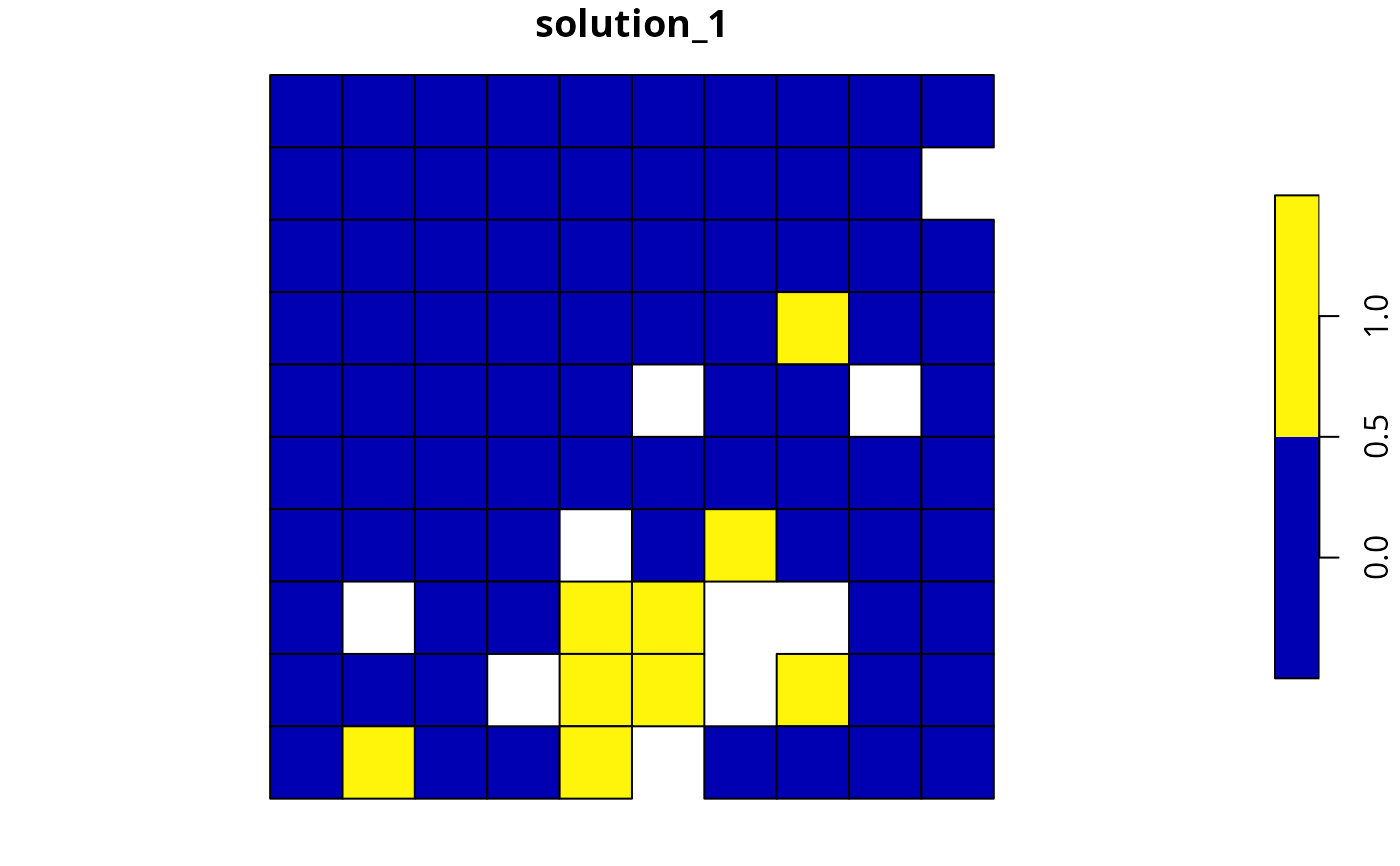
# plot solution
plot(s2[, "solution_1"])
# calculate boundary associated with the solution
r1 <- eval_boundary_summary(p1, s1)
print(r1)
#> # A tibble: 1 × 2
#> summary boundary
#> <chr> <dbl>
#> 1 overall 2.25
# build minimal conservation problem with polygon data
p2 <-
problem(sim_pu_polygons, sim_features, cost_column = "cost") %>%
add_min_set_objective() %>%
add_relative_targets(0.1) %>%
add_binary_decisions() %>%
add_default_solver(verbose = FALSE)
# solve the problem
s2 <- solve(p2)
# print solution
print(s2)
#> Simple feature collection with 90 features and 4 fields
#> Geometry type: POLYGON
#> Dimension: XY
#> Bounding box: xmin: 0 ymin: 0 xmax: 1 ymax: 1
#> Projected CRS: WGS 84 / Pseudo-Mercator
#> # A tibble: 90 × 5
#> cost locked_in locked_out solution_1 geometry
#> * <dbl> <lgl> <lgl> <dbl> <POLYGON [m]>
#> 1 216. FALSE FALSE 0 ((0 1, 0.1 1, 0.1 0.9, 0 0.9, 0 1))
#> 2 213. FALSE FALSE 0 ((0.1 1, 0.2 1, 0.2 0.9, 0.1 0.9, 0.1 …
#> 3 207. FALSE FALSE 0 ((0.2 1, 0.3 1, 0.3 0.9, 0.2 0.9, 0.2 …
#> 4 209. FALSE TRUE 0 ((0.3 1, 0.4 1, 0.4 0.9, 0.3 0.9, 0.3 …
#> 5 214. FALSE FALSE 0 ((0.4 1, 0.5 1, 0.5 0.9, 0.4 0.9, 0.4 …
#> 6 214. FALSE FALSE 0 ((0.5 1, 0.6 1, 0.6 0.9, 0.5 0.9, 0.5 …
#> 7 210. FALSE FALSE 0 ((0.6 1, 0.7 1, 0.7 0.9, 0.6 0.9, 0.6 …
#> 8 211. FALSE TRUE 0 ((0.7 1, 0.8 1, 0.8 0.9, 0.7 0.9, 0.7 …
#> 9 210. FALSE FALSE 0 ((0.8 1, 0.9 1, 0.9 0.9, 0.8 0.9, 0.8 …
#> 10 204. FALSE FALSE 0 ((0.9 1, 1 1, 1 0.9, 0.9 0.9, 0.9 1))
#> # ℹ 80 more rows
# plot solution
plot(s2[, "solution_1"])
 # calculate boundary associated with the solution
r2 <- eval_boundary_summary(p2, s2[, "solution_1"])
print(r2)
#> # A tibble: 1 × 2
#> summary boundary
#> <chr> <dbl>
#> 1 overall 2.05
# build multi-zone conservation problem with polygon data
p3 <-
problem(
sim_zones_pu_polygons, sim_zones_features,
cost_column = c("cost_1", "cost_2", "cost_3")
) %>%
add_min_set_objective() %>%
add_relative_targets(matrix(runif(15, 0.1, 0.2), nrow = 5, ncol = 3)) %>%
add_binary_decisions() %>%
add_default_solver(verbose = FALSE)
# solve the problem
s3 <- solve(p3)
# print solution
print(s3)
#> Simple feature collection with 90 features and 9 fields
#> Geometry type: POLYGON
#> Dimension: XY
#> Bounding box: xmin: 0 ymin: 0 xmax: 1 ymax: 1
#> Projected CRS: WGS 84 / Pseudo-Mercator
#> # A tibble: 90 × 10
#> cost_1 cost_2 cost_3 locked_1 locked_2 locked_3 solution_1_zone_1
#> * <dbl> <dbl> <dbl> <lgl> <lgl> <lgl> <dbl>
#> 1 216. 183. 205. FALSE FALSE FALSE 0
#> 2 213. 189. 210. FALSE FALSE FALSE 0
#> 3 207. 194. 215. TRUE FALSE FALSE 0
#> 4 209. 198. 219. FALSE FALSE FALSE 0
#> 5 214. 200. 221. FALSE FALSE FALSE 0
#> 6 214. 203. 225. FALSE FALSE FALSE 0
#> 7 211. 209. 223. FALSE FALSE FALSE 0
#> 8 210. 212. 222. TRUE FALSE FALSE 0
#> 9 204. 218. 214. FALSE FALSE FALSE 0
#> 10 213. 183. 206. FALSE FALSE FALSE 0
#> # ℹ 80 more rows
#> # ℹ 3 more variables: solution_1_zone_2 <dbl>, solution_1_zone_3 <dbl>,
#> # geometry <POLYGON [m]>
# create new column representing the zone id that each planning unit
# was allocated to in the solution
s3$solution <- category_vector(
s3[, c("solution_1_zone_1", "solution_1_zone_2", "solution_1_zone_3")]
)
s3$solution <- factor(s3$solution)
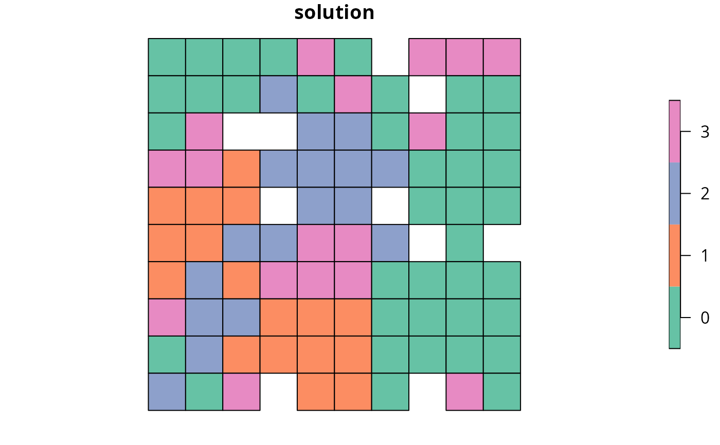
# plot solution
plot(s3[, "solution"])
# calculate boundary associated with the solution
r2 <- eval_boundary_summary(p2, s2[, "solution_1"])
print(r2)
#> # A tibble: 1 × 2
#> summary boundary
#> <chr> <dbl>
#> 1 overall 2.05
# build multi-zone conservation problem with polygon data
p3 <-
problem(
sim_zones_pu_polygons, sim_zones_features,
cost_column = c("cost_1", "cost_2", "cost_3")
) %>%
add_min_set_objective() %>%
add_relative_targets(matrix(runif(15, 0.1, 0.2), nrow = 5, ncol = 3)) %>%
add_binary_decisions() %>%
add_default_solver(verbose = FALSE)
# solve the problem
s3 <- solve(p3)
# print solution
print(s3)
#> Simple feature collection with 90 features and 9 fields
#> Geometry type: POLYGON
#> Dimension: XY
#> Bounding box: xmin: 0 ymin: 0 xmax: 1 ymax: 1
#> Projected CRS: WGS 84 / Pseudo-Mercator
#> # A tibble: 90 × 10
#> cost_1 cost_2 cost_3 locked_1 locked_2 locked_3 solution_1_zone_1
#> * <dbl> <dbl> <dbl> <lgl> <lgl> <lgl> <dbl>
#> 1 216. 183. 205. FALSE FALSE FALSE 0
#> 2 213. 189. 210. FALSE FALSE FALSE 0
#> 3 207. 194. 215. TRUE FALSE FALSE 0
#> 4 209. 198. 219. FALSE FALSE FALSE 0
#> 5 214. 200. 221. FALSE FALSE FALSE 0
#> 6 214. 203. 225. FALSE FALSE FALSE 0
#> 7 211. 209. 223. FALSE FALSE FALSE 0
#> 8 210. 212. 222. TRUE FALSE FALSE 0
#> 9 204. 218. 214. FALSE FALSE FALSE 0
#> 10 213. 183. 206. FALSE FALSE FALSE 0
#> # ℹ 80 more rows
#> # ℹ 3 more variables: solution_1_zone_2 <dbl>, solution_1_zone_3 <dbl>,
#> # geometry <POLYGON [m]>
# create new column representing the zone id that each planning unit
# was allocated to in the solution
s3$solution <- category_vector(
s3[, c("solution_1_zone_1", "solution_1_zone_2", "solution_1_zone_3")]
)
s3$solution <- factor(s3$solution)
# plot solution
plot(s3[, "solution"])
 # calculate boundary associated with the solution
# here we will use the default argument for zones which treats each
# zone as completely separate, meaning that the "overall"
# boundary is just the sum of the boundaries for each zone
r3 <- eval_boundary_summary(
p3, s3[, c("solution_1_zone_1", "solution_1_zone_2", "solution_1_zone_3")]
)
print(r3)
#> # A tibble: 4 × 2
#> summary boundary
#> <chr> <dbl>
#> 1 overall 10.6
#> 2 zone_1 2.75
#> 3 zone_2 3.6
#> 4 zone_3 4.25
# let's calculate the overall exposed boundary across the entire
# solution, assuming that the shared boundaries between planning
# units allocated to different zones "count" just as much
# as those for planning units allocated to the same zone
# in other words, let's calculate the overall exposed boundary
# across the entire solution by "combining" all selected planning units
# together (regardless of which zone they are allocated to in the solution)
r3_combined <- eval_boundary_summary(
p3, zones = matrix(1, ncol = 3, nrow = 3),
s3[, c("solution_1_zone_1", "solution_1_zone_2", "solution_1_zone_3")]
)
print(r3_combined)
#> # A tibble: 4 × 2
#> summary boundary
#> <chr> <dbl>
#> 1 overall 5.20
#> 2 zone_1 2.75
#> 3 zone_2 3.6
#> 4 zone_3 4.25
# we can see that the "overall" boundary is now less than the
# sum of the individual zone boundaries, because it does not
# consider the shared boundary between two planning units allocated to
# different zones as "exposed" when performing the calculations
# calculate boundary associated with the solution
# here we will use the default argument for zones which treats each
# zone as completely separate, meaning that the "overall"
# boundary is just the sum of the boundaries for each zone
r3 <- eval_boundary_summary(
p3, s3[, c("solution_1_zone_1", "solution_1_zone_2", "solution_1_zone_3")]
)
print(r3)
#> # A tibble: 4 × 2
#> summary boundary
#> <chr> <dbl>
#> 1 overall 10.6
#> 2 zone_1 2.75
#> 3 zone_2 3.6
#> 4 zone_3 4.25
# let's calculate the overall exposed boundary across the entire
# solution, assuming that the shared boundaries between planning
# units allocated to different zones "count" just as much
# as those for planning units allocated to the same zone
# in other words, let's calculate the overall exposed boundary
# across the entire solution by "combining" all selected planning units
# together (regardless of which zone they are allocated to in the solution)
r3_combined <- eval_boundary_summary(
p3, zones = matrix(1, ncol = 3, nrow = 3),
s3[, c("solution_1_zone_1", "solution_1_zone_2", "solution_1_zone_3")]
)
print(r3_combined)
#> # A tibble: 4 × 2
#> summary boundary
#> <chr> <dbl>
#> 1 overall 5.20
#> 2 zone_1 2.75
#> 3 zone_2 3.6
#> 4 zone_3 4.25
# we can see that the "overall" boundary is now less than the
# sum of the individual zone boundaries, because it does not
# consider the shared boundary between two planning units allocated to
# different zones as "exposed" when performing the calculations