Calculate the number of planning units selected within a solution to a conservation planning problem.
Arguments
- x
problem()ormulti_problem()object.- solution
numeric,matrix,data.frame,terra::rast(), orsf::sf()object. Note thatsolutionmust have the same format as the planning unit data inx. See the Solution format section for more information.
Value
A tibble::tibble() object containing the number of planning
units selected within a solution.
It contains the following columns.
- summary
characterdescription of the summary statistic. The statistic associated with the"overall"value in this column is calculated using the entire solution (including all management zones ifxhas multiple zones). Ifxhas multiple management zones, then summary statistics are also provided for each zone separately (indicated using zone names).- n
numericnumber of selected planning units.
Details
This summary statistic is calculated as the sum of the values in
the solution. As a consequence, this metric can produce a
non-integer value (e.g., 4.3) for solutions containing proportion values
(e.g., generated by solving a problem() built using the
add_proportion_decisions() function).
Solution format
Broadly speaking, solution must be in the same format as
the planning unit data in x.
Further details on the correct format are listed separately
for each of the different planning unit data formats.
xhasnumericplanning unitsHere
solutionmust be anumericvector with each element corresponding to a different planning unit. It should have the same number of planning units as those inx. Additionally, any planning units with missing cost (NA) values should also have missing (NA) values in thesolution.xhasmatrixplanning unitsHere
solutionmust be amatrixvector with each row corresponding to a different planning unit, and each column correspond to a different management zone. It should have the same number of planning units and zones as those inx. Additionally, any planning units with missing cost (NA) values for a particular zone should also have a missing (NA) values insolution.xhasterra::rast()planning unitsHere
solutionbe aterra::rast()object where different cells correspond to different planning units and layers correspond to a different management zones. It should have the same dimensionality (rows, columns, layers), resolution, extent, and coordinate reference system as the planning units inx. Additionally, any planning units with missing cost (NA) values for a particular zone should also have missing (NA) values insolution.xhasdata.frameplanning unitsHere
solutionmust be adata.framewith each column corresponding to a different zone, each row corresponding to a different planning unit, and cell values corresponding to the solution value. This means that if adata.frameobject containing the solution also contains additional columns, then these columns will need to be subsetted prior to using this function (see below for example withsf::sf()data). Additionally, any planning units with missing cost (NA) values for a particular zone should also have missing (NA) values insolution.xhassf::sf()planning unitsHere
solutionmust be asf::sf()object with each column corresponding to a different zone, each row corresponding to a different planning unit, and cell values corresponding to the solution value. This means that if thesf::sf()object containing the solution also contains additional columns, then these columns will need to be subsetted prior to using this function (see below for example). Additionally,solutionmust also have the same coordinate reference system as the planning unit data. Furthermore, any planning units with missing cost (NA) values for a particular zone should also have missing (NA) values insolution.
See also
See summaries for an overview of all functions for summarizing solutions.
Other functions for summarizing solutions:
eval_asym_connectivity_summary(),
eval_boundary_summary(),
eval_connectivity_summary(),
eval_cost_summary(),
eval_feature_representation_summary(),
eval_objective_summary(),
eval_target_coverage_summary()
Examples
# set seed for reproducibility
set.seed(500)
# load data
sim_pu_raster <- get_sim_pu_raster()
sim_pu_polygons <- get_sim_pu_polygons()
sim_features <- get_sim_features()
sim_zones_pu_polygons <- get_sim_zones_pu_polygons()
sim_zones_features <- get_sim_zones_features()
# build minimal conservation problem with raster data
p1 <-
problem(sim_pu_raster, sim_features) %>%
add_min_set_objective() %>%
add_relative_targets(0.1) %>%
add_binary_decisions() %>%
add_default_solver(verbose = FALSE)
# solve the problem
s1 <- solve(p1)
# print solution
print(s1)
#> class : SpatRaster
#> size : 10, 10, 1 (nrow, ncol, nlyr)
#> resolution : 0.1, 0.1 (x, y)
#> extent : 0, 1, 0, 1 (xmin, xmax, ymin, ymax)
#> coord. ref. : WGS 84 / Pseudo-Mercator (EPSG:3857)
#> source(s) : memory
#> varname : sim_pu_raster
#> name : layer
#> min value : 0
#> max value : 1
# plot solution
plot(s1, main = "solution", axes = FALSE)
 # calculate number of selected planning units within solution
r1 <- eval_n_summary(p1, s1)
print(r1)
#> # A tibble: 1 × 2
#> summary n
#> <chr> <dbl>
#> 1 overall 10
# build minimal conservation problem with polygon data
p2 <-
problem(sim_pu_polygons, sim_features, cost_column = "cost") %>%
add_min_set_objective() %>%
add_relative_targets(0.1) %>%
add_binary_decisions() %>%
add_default_solver(verbose = FALSE)
# solve the problem
s2 <- solve(p2)
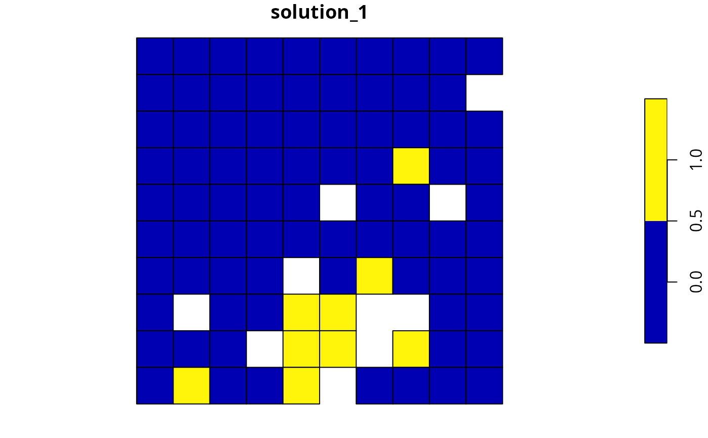
# plot solution
plot(s2[, "solution_1"])
# calculate number of selected planning units within solution
r1 <- eval_n_summary(p1, s1)
print(r1)
#> # A tibble: 1 × 2
#> summary n
#> <chr> <dbl>
#> 1 overall 10
# build minimal conservation problem with polygon data
p2 <-
problem(sim_pu_polygons, sim_features, cost_column = "cost") %>%
add_min_set_objective() %>%
add_relative_targets(0.1) %>%
add_binary_decisions() %>%
add_default_solver(verbose = FALSE)
# solve the problem
s2 <- solve(p2)
# plot solution
plot(s2[, "solution_1"])
 # print solution
print(s2)
#> Simple feature collection with 90 features and 4 fields
#> Geometry type: POLYGON
#> Dimension: XY
#> Bounding box: xmin: 0 ymin: 0 xmax: 1 ymax: 1
#> Projected CRS: WGS 84 / Pseudo-Mercator
#> # A tibble: 90 × 5
#> cost locked_in locked_out solution_1 geometry
#> * <dbl> <lgl> <lgl> <dbl> <POLYGON [m]>
#> 1 216. FALSE FALSE 0 ((0 1, 0.1 1, 0.1 0.9, 0 0.9, 0 1))
#> 2 213. FALSE FALSE 0 ((0.1 1, 0.2 1, 0.2 0.9, 0.1 0.9, 0.1 …
#> 3 207. FALSE FALSE 0 ((0.2 1, 0.3 1, 0.3 0.9, 0.2 0.9, 0.2 …
#> 4 209. FALSE TRUE 0 ((0.3 1, 0.4 1, 0.4 0.9, 0.3 0.9, 0.3 …
#> 5 214. FALSE FALSE 0 ((0.4 1, 0.5 1, 0.5 0.9, 0.4 0.9, 0.4 …
#> 6 214. FALSE FALSE 0 ((0.5 1, 0.6 1, 0.6 0.9, 0.5 0.9, 0.5 …
#> 7 210. FALSE FALSE 0 ((0.6 1, 0.7 1, 0.7 0.9, 0.6 0.9, 0.6 …
#> 8 211. FALSE TRUE 0 ((0.7 1, 0.8 1, 0.8 0.9, 0.7 0.9, 0.7 …
#> 9 210. FALSE FALSE 0 ((0.8 1, 0.9 1, 0.9 0.9, 0.8 0.9, 0.8 …
#> 10 204. FALSE FALSE 0 ((0.9 1, 1 1, 1 0.9, 0.9 0.9, 0.9 1))
#> # ℹ 80 more rows
# calculate number of selected planning units within solution
r2 <- eval_n_summary(p2, s2[, "solution_1"])
print(r2)
#> # A tibble: 1 × 2
#> summary n
#> <chr> <dbl>
#> 1 overall 9
# manually calculate number of selected planning units
r2_manual <- sum(s2$solution_1, na.rm = TRUE)
print(r2_manual)
#> [1] 9
# build multi-zone conservation problem with polygon data
p3 <-
problem(
sim_zones_pu_polygons, sim_zones_features,
cost_column = c("cost_1", "cost_2", "cost_3")
) %>%
add_min_set_objective() %>%
add_relative_targets(matrix(runif(15, 0.1, 0.2), nrow = 5, ncol = 3)) %>%
add_binary_decisions() %>%
add_default_solver(verbose = FALSE)
# solve the problem
s3 <- solve(p3)
# print solution
print(s3)
#> Simple feature collection with 90 features and 9 fields
#> Geometry type: POLYGON
#> Dimension: XY
#> Bounding box: xmin: 0 ymin: 0 xmax: 1 ymax: 1
#> Projected CRS: WGS 84 / Pseudo-Mercator
#> # A tibble: 90 × 10
#> cost_1 cost_2 cost_3 locked_1 locked_2 locked_3 solution_1_zone_1
#> * <dbl> <dbl> <dbl> <lgl> <lgl> <lgl> <dbl>
#> 1 216. 183. 205. FALSE FALSE FALSE 0
#> 2 213. 189. 210. FALSE FALSE FALSE 0
#> 3 207. 194. 215. TRUE FALSE FALSE 0
#> 4 209. 198. 219. FALSE FALSE FALSE 0
#> 5 214. 200. 221. FALSE FALSE FALSE 0
#> 6 214. 203. 225. FALSE FALSE FALSE 0
#> 7 211. 209. 223. FALSE FALSE FALSE 0
#> 8 210. 212. 222. TRUE FALSE FALSE 0
#> 9 204. 218. 214. FALSE FALSE FALSE 0
#> 10 213. 183. 206. FALSE FALSE FALSE 0
#> # ℹ 80 more rows
#> # ℹ 3 more variables: solution_1_zone_2 <dbl>, solution_1_zone_3 <dbl>,
#> # geometry <POLYGON [m]>
# create new column representing the zone id that each planning unit
# was allocated to in the solution
s3$solution <- category_vector(
s3[, c("solution_1_zone_1", "solution_1_zone_2", "solution_1_zone_3")]
)
s3$solution <- factor(s3$solution)
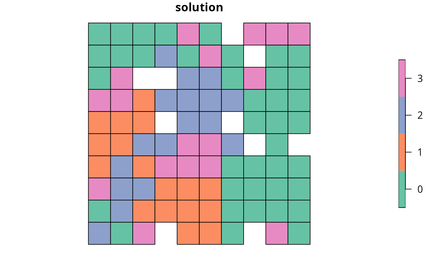
# plot solution
plot(s3[, "solution"])
# print solution
print(s2)
#> Simple feature collection with 90 features and 4 fields
#> Geometry type: POLYGON
#> Dimension: XY
#> Bounding box: xmin: 0 ymin: 0 xmax: 1 ymax: 1
#> Projected CRS: WGS 84 / Pseudo-Mercator
#> # A tibble: 90 × 5
#> cost locked_in locked_out solution_1 geometry
#> * <dbl> <lgl> <lgl> <dbl> <POLYGON [m]>
#> 1 216. FALSE FALSE 0 ((0 1, 0.1 1, 0.1 0.9, 0 0.9, 0 1))
#> 2 213. FALSE FALSE 0 ((0.1 1, 0.2 1, 0.2 0.9, 0.1 0.9, 0.1 …
#> 3 207. FALSE FALSE 0 ((0.2 1, 0.3 1, 0.3 0.9, 0.2 0.9, 0.2 …
#> 4 209. FALSE TRUE 0 ((0.3 1, 0.4 1, 0.4 0.9, 0.3 0.9, 0.3 …
#> 5 214. FALSE FALSE 0 ((0.4 1, 0.5 1, 0.5 0.9, 0.4 0.9, 0.4 …
#> 6 214. FALSE FALSE 0 ((0.5 1, 0.6 1, 0.6 0.9, 0.5 0.9, 0.5 …
#> 7 210. FALSE FALSE 0 ((0.6 1, 0.7 1, 0.7 0.9, 0.6 0.9, 0.6 …
#> 8 211. FALSE TRUE 0 ((0.7 1, 0.8 1, 0.8 0.9, 0.7 0.9, 0.7 …
#> 9 210. FALSE FALSE 0 ((0.8 1, 0.9 1, 0.9 0.9, 0.8 0.9, 0.8 …
#> 10 204. FALSE FALSE 0 ((0.9 1, 1 1, 1 0.9, 0.9 0.9, 0.9 1))
#> # ℹ 80 more rows
# calculate number of selected planning units within solution
r2 <- eval_n_summary(p2, s2[, "solution_1"])
print(r2)
#> # A tibble: 1 × 2
#> summary n
#> <chr> <dbl>
#> 1 overall 9
# manually calculate number of selected planning units
r2_manual <- sum(s2$solution_1, na.rm = TRUE)
print(r2_manual)
#> [1] 9
# build multi-zone conservation problem with polygon data
p3 <-
problem(
sim_zones_pu_polygons, sim_zones_features,
cost_column = c("cost_1", "cost_2", "cost_3")
) %>%
add_min_set_objective() %>%
add_relative_targets(matrix(runif(15, 0.1, 0.2), nrow = 5, ncol = 3)) %>%
add_binary_decisions() %>%
add_default_solver(verbose = FALSE)
# solve the problem
s3 <- solve(p3)
# print solution
print(s3)
#> Simple feature collection with 90 features and 9 fields
#> Geometry type: POLYGON
#> Dimension: XY
#> Bounding box: xmin: 0 ymin: 0 xmax: 1 ymax: 1
#> Projected CRS: WGS 84 / Pseudo-Mercator
#> # A tibble: 90 × 10
#> cost_1 cost_2 cost_3 locked_1 locked_2 locked_3 solution_1_zone_1
#> * <dbl> <dbl> <dbl> <lgl> <lgl> <lgl> <dbl>
#> 1 216. 183. 205. FALSE FALSE FALSE 0
#> 2 213. 189. 210. FALSE FALSE FALSE 0
#> 3 207. 194. 215. TRUE FALSE FALSE 0
#> 4 209. 198. 219. FALSE FALSE FALSE 0
#> 5 214. 200. 221. FALSE FALSE FALSE 0
#> 6 214. 203. 225. FALSE FALSE FALSE 0
#> 7 211. 209. 223. FALSE FALSE FALSE 0
#> 8 210. 212. 222. TRUE FALSE FALSE 0
#> 9 204. 218. 214. FALSE FALSE FALSE 0
#> 10 213. 183. 206. FALSE FALSE FALSE 0
#> # ℹ 80 more rows
#> # ℹ 3 more variables: solution_1_zone_2 <dbl>, solution_1_zone_3 <dbl>,
#> # geometry <POLYGON [m]>
# create new column representing the zone id that each planning unit
# was allocated to in the solution
s3$solution <- category_vector(
s3[, c("solution_1_zone_1", "solution_1_zone_2", "solution_1_zone_3")]
)
s3$solution <- factor(s3$solution)
# plot solution
plot(s3[, "solution"])
 # calculate number of selected planning units within solution
r3 <- eval_n_summary(
p3, s3[, c("solution_1_zone_1", "solution_1_zone_2", "solution_1_zone_3")]
)
print(r3)
#> # A tibble: 4 × 2
#> summary n
#> <chr> <dbl>
#> 1 overall 51
#> 2 zone_1 17
#> 3 zone_2 17
#> 4 zone_3 17
# calculate number of selected planning units within solution
r3 <- eval_n_summary(
p3, s3[, c("solution_1_zone_1", "solution_1_zone_2", "solution_1_zone_3")]
)
print(r3)
#> # A tibble: 4 × 2
#> summary n
#> <chr> <dbl>
#> 1 overall 51
#> 2 zone_1 17
#> 3 zone_2 17
#> 4 zone_3 17