Evaluate feature representation by solution
Source:R/eval_feature_representation_summary.R
eval_feature_representation_summary.RdCalculate how well features are represented by a solution to a conservation planning problem. These summary statistics are reported for each and every feature, and each and every zone, within a conservation planning problem.
Usage
eval_feature_representation_summary(x, solution)

# S3 method for class 'ConservationProblem'
eval_feature_representation_summary(x, solution)

# S3 method for class 'MultiConservationProblem'
eval_feature_representation_summary(x, solution)
Arguments
- x
problem()ormulti_problem()object.- solution
numeric,matrix,data.frame,terra::rast(), orsf::sf()object. Note thatsolutionmust have the same format as the planning unit data inx. See the Solution format section for more information.
Value
A tibble::tibble() object describing feature representation by the
solution.
Here, each row describes a specific summary statistic
(e.g., different management zone) for a specific feature.
It contains the following columns.
- problem
charactername of problem. Note that this column is only present ifxis amulti_problem()object.- summary
characterdescription of the summary statistic. The statistics associated with the"overall"value in this column are calculated using all planning unit values. Ifxhas multiple management zones, this means that all calculations are completed by summing together all planning unit values across all zones. For example, if there are two zones, a single planning unit, and a feature has a value of one in the single planning unit for both zones, thentotal_amountwill contain a value of two (even though it would not be possible to to achieve a value of two because the planning unit could not simultaneously be allocated to both zones). Additionally, ifxhas multiple management zones, then summary statistics are also provided for each zone separately (indicated using zone names).- feature
charactername of the feature.- total_amount
numerictotal amount of each feature available in the entire conservation planning problem (not just planning units selected within the solution). It is calculated as the sum of the feature data, supplied when creating aproblem()object (e.g., presence/absence values).- absolute_held
numerictotal amount of each feature secured within the solution. It is calculated as the sum of the feature data, supplied when creating aproblem()object (e.g., presence/absence values), weighted by the status of each planning unit in the solution (e.g., selected or not for prioritization).- relative_held
numericproportion of each feature secured within the solution. It is calculated by dividing values in the"absolute_held"column by those in the"total_amount"column.
Solution format
Broadly speaking, solution must be in the same format as
the planning unit data in x.
Further details on the correct format are listed separately
for each of the different planning unit data formats.
xhasnumericplanning unitsHere
solutionmust be anumericvector with each element corresponding to a different planning unit. It should have the same number of planning units as those inx. Additionally, any planning units with missing cost (NA) values should also have missing (NA) values in thesolution.xhasmatrixplanning unitsHere
solutionmust be amatrixvector with each row corresponding to a different planning unit, and each column correspond to a different management zone. It should have the same number of planning units and zones as those inx. Additionally, any planning units with missing cost (NA) values for a particular zone should also have a missing (NA) values insolution.xhasterra::rast()planning unitsHere
solutionbe aterra::rast()object where different cells correspond to different planning units and layers correspond to a different management zones. It should have the same dimensionality (rows, columns, layers), resolution, extent, and coordinate reference system as the planning units inx. Additionally, any planning units with missing cost (NA) values for a particular zone should also have missing (NA) values insolution.xhasdata.frameplanning unitsHere
solutionmust be adata.framewith each column corresponding to a different zone, each row corresponding to a different planning unit, and cell values corresponding to the solution value. This means that if adata.frameobject containing the solution also contains additional columns, then these columns will need to be subsetted prior to using this function (see below for example withsf::sf()data). Additionally, any planning units with missing cost (NA) values for a particular zone should also have missing (NA) values insolution.xhassf::sf()planning unitsHere
solutionmust be asf::sf()object with each column corresponding to a different zone, each row corresponding to a different planning unit, and cell values corresponding to the solution value. This means that if thesf::sf()object containing the solution also contains additional columns, then these columns will need to be subsetted prior to using this function (see below for example). Additionally,solutionmust also have the same coordinate reference system as the planning unit data. Furthermore, any planning units with missing cost (NA) values for a particular zone should also have missing (NA) values insolution.
See also
See summaries for an overview of all functions for summarizing solutions.
Other functions for summarizing solutions:
eval_asym_connectivity_summary(),
eval_boundary_summary(),
eval_connectivity_summary(),
eval_cost_summary(),
eval_n_summary(),
eval_objective_summary(),
eval_target_coverage_summary()
Examples
# set seed for reproducibility
set.seed(500)
# load data
sim_pu_raster <- get_sim_pu_raster()
sim_pu_polygons <- get_sim_pu_polygons()
sim_features <- get_sim_features()
sim_zones_pu_raster <- get_sim_zones_pu_raster()
sim_zones_pu_polygons <- get_sim_zones_pu_polygons()
sim_zones_features <- get_sim_zones_features()
# create a simple conservation planning dataset so we can see exactly
# how feature representation is calculated
pu <- data.frame(
id = seq_len(10),
cost = c(0.2, NA, runif(8)),
spp1 = runif(10),
spp2 = c(rpois(9, 4), NA)
)
# create problem
p1 <-
problem(pu, c("spp1", "spp2"), cost_column = "cost") %>%
add_min_set_objective() %>%
add_relative_targets(0.1) %>%
add_binary_decisions() %>%
add_default_solver(verbose = FALSE)
# create a solution
# specifically, a data.frame with a single column that contains
# binary values indicating if each planning units was selected or not
s1 <- data.frame(s = c(1, NA, rep(c(1, 0), 4)))
print(s1)
#> s
#> 1 1
#> 2 NA
#> 3 1
#> 4 0
#> 5 1
#> 6 0
#> 7 1
#> 8 0
#> 9 1
#> 10 0
# calculate feature representation
r1 <- eval_feature_representation_summary(p1, s1)
print(r1)
#> # A tibble: 2 × 5
#> summary feature total_amount absolute_held relative_held
#> <chr> <chr> <dbl> <dbl> <dbl>
#> 1 overall spp1 5.76 3.12 0.541
#> 2 overall spp2 33 14 0.424
# let's verify that feature representation calculations are correct
# by manually performing the calculations and compare the results with r1
## calculate total amount for each feature
print(
setNames(
c(sum(pu$spp1, na.rm = TRUE), sum(pu$spp2, na.rm = TRUE)),
c("spp1", "spp2")
)
)
#> spp1 spp2
#> 5.755739 33.000000
## calculate absolute amount held for each feature
print(
setNames(
c(sum(pu$spp1 * s1$s, na.rm = TRUE), sum(pu$spp2 * s1$s, na.rm = TRUE)),
c("spp1", "spp2")
)
)
#> spp1 spp2
#> 3.116052 14.000000
## calculate relative amount held for each feature
print(
setNames(
c(
sum(pu$spp1 * s1$s, na.rm = TRUE) / sum(pu$spp1, na.rm = TRUE),
sum(pu$spp2 * s1$s, na.rm = TRUE) / sum(pu$spp2, na.rm = TRUE)
),
c("spp1", "spp2")
)
)
#> spp1 spp2
#> 0.5413818 0.4242424
# solve problem using an exact algorithm solver
s1_2 <- solve(p1)
print(s1_2)
#> # A tibble: 10 × 5
#> id cost spp1 spp2 solution_1
#> <int> <dbl> <dbl> <int> <dbl>
#> 1 1 0.2 0.829 4 1
#> 2 2 NA 0.712 3 NA
#> 3 3 0.834 0.282 1 0
#> 4 4 0.725 0.893 6 0
#> 5 5 0.975 0.765 1 0
#> 6 6 0.468 0.164 4 0
#> 7 7 0.812 0.732 3 0
#> 8 8 0.206 0.253 6 0
#> 9 9 0.512 0.508 5 0
#> 10 10 0.925 0.618 NA 0
# calculate feature representation in this solution
r1_2 <- eval_feature_representation_summary(
p1, s1_2[, "solution_1", drop = FALSE]
)
print(r1_2)
#> # A tibble: 2 × 5
#> summary feature total_amount absolute_held relative_held
#> <chr> <chr> <dbl> <dbl> <dbl>
#> 1 overall spp1 5.76 0.829 0.144
#> 2 overall spp2 33 4 0.121
# build minimal conservation problem with raster data
p2 <-
problem(sim_pu_raster, sim_features) %>%
add_min_set_objective() %>%
add_relative_targets(0.1) %>%
add_binary_decisions() %>%
add_default_solver(verbose = FALSE)
# solve problem
s2 <- solve(p2)
# print solution
print(s2)
#> class : SpatRaster
#> size : 10, 10, 1 (nrow, ncol, nlyr)
#> resolution : 0.1, 0.1 (x, y)
#> extent : 0, 1, 0, 1 (xmin, xmax, ymin, ymax)
#> coord. ref. : WGS 84 / Pseudo-Mercator (EPSG:3857)
#> source(s) : memory
#> varname : sim_pu_raster
#> name : layer
#> min value : 0
#> max value : 1
# calculate feature representation in the solution
r2 <- eval_feature_representation_summary(p2, s2)
print(r2)
#> # A tibble: 5 × 5
#> summary feature total_amount absolute_held relative_held
#> <chr> <chr> <dbl> <dbl> <dbl>
#> 1 overall feature_1 83.3 8.91 0.107
#> 2 overall feature_2 31.2 3.13 0.100
#> 3 overall feature_3 72.0 7.34 0.102
#> 4 overall feature_4 42.7 4.35 0.102
#> 5 overall feature_5 56.7 6.01 0.106
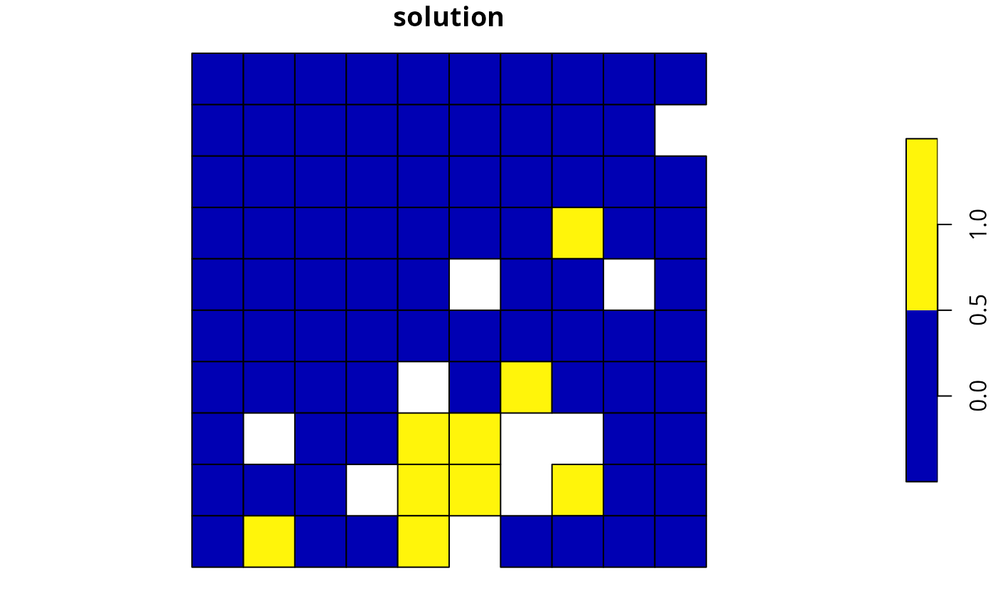
# plot solution
plot(s2, main = "solution", axes = FALSE)
 # build minimal conservation problem with polygon data
p3 <-
problem(sim_pu_polygons, sim_features, cost_column = "cost") %>%
add_min_set_objective() %>%
add_relative_targets(0.1) %>%
add_binary_decisions() %>%
add_default_solver(verbose = FALSE)
# solve problem
s3 <- solve(p3)
# print first six rows of the attribute table
print(head(s3))
#> Simple feature collection with 6 features and 4 fields
#> Geometry type: POLYGON
#> Dimension: XY
#> Bounding box: xmin: 0 ymin: 0.9 xmax: 0.6 ymax: 1
#> Projected CRS: WGS 84 / Pseudo-Mercator
#> # A tibble: 6 × 5
#> cost locked_in locked_out solution_1 geometry
#> <dbl> <lgl> <lgl> <dbl> <POLYGON [m]>
#> 1 216. FALSE FALSE 0 ((0 1, 0.1 1, 0.1 0.9, 0 0.9, 0 1))
#> 2 213. FALSE FALSE 0 ((0.1 1, 0.2 1, 0.2 0.9, 0.1 0.9, 0.1 1…
#> 3 207. FALSE FALSE 0 ((0.2 1, 0.3 1, 0.3 0.9, 0.2 0.9, 0.2 1…
#> 4 209. FALSE TRUE 0 ((0.3 1, 0.4 1, 0.4 0.9, 0.3 0.9, 0.3 1…
#> 5 214. FALSE FALSE 0 ((0.4 1, 0.5 1, 0.5 0.9, 0.4 0.9, 0.4 1…
#> 6 214. FALSE FALSE 0 ((0.5 1, 0.6 1, 0.6 0.9, 0.5 0.9, 0.5 1…
# calculate feature representation in the solution
r3 <- eval_feature_representation_summary(p3, s3[, "solution_1"])
print(r3)
#> # A tibble: 5 × 5
#> summary feature total_amount absolute_held relative_held
#> <chr> <chr> <dbl> <dbl> <dbl>
#> 1 overall feature_1 74.5 8.05 0.108
#> 2 overall feature_2 28.1 2.83 0.101
#> 3 overall feature_3 64.9 6.65 0.103
#> 4 overall feature_4 38.2 3.87 0.101
#> 5 overall feature_5 50.7 5.41 0.107
# plot solution
plot(s3[, "solution_1"], main = "solution", axes = FALSE)
# build minimal conservation problem with polygon data
p3 <-
problem(sim_pu_polygons, sim_features, cost_column = "cost") %>%
add_min_set_objective() %>%
add_relative_targets(0.1) %>%
add_binary_decisions() %>%
add_default_solver(verbose = FALSE)
# solve problem
s3 <- solve(p3)
# print first six rows of the attribute table
print(head(s3))
#> Simple feature collection with 6 features and 4 fields
#> Geometry type: POLYGON
#> Dimension: XY
#> Bounding box: xmin: 0 ymin: 0.9 xmax: 0.6 ymax: 1
#> Projected CRS: WGS 84 / Pseudo-Mercator
#> # A tibble: 6 × 5
#> cost locked_in locked_out solution_1 geometry
#> <dbl> <lgl> <lgl> <dbl> <POLYGON [m]>
#> 1 216. FALSE FALSE 0 ((0 1, 0.1 1, 0.1 0.9, 0 0.9, 0 1))
#> 2 213. FALSE FALSE 0 ((0.1 1, 0.2 1, 0.2 0.9, 0.1 0.9, 0.1 1…
#> 3 207. FALSE FALSE 0 ((0.2 1, 0.3 1, 0.3 0.9, 0.2 0.9, 0.2 1…
#> 4 209. FALSE TRUE 0 ((0.3 1, 0.4 1, 0.4 0.9, 0.3 0.9, 0.3 1…
#> 5 214. FALSE FALSE 0 ((0.4 1, 0.5 1, 0.5 0.9, 0.4 0.9, 0.4 1…
#> 6 214. FALSE FALSE 0 ((0.5 1, 0.6 1, 0.6 0.9, 0.5 0.9, 0.5 1…
# calculate feature representation in the solution
r3 <- eval_feature_representation_summary(p3, s3[, "solution_1"])
print(r3)
#> # A tibble: 5 × 5
#> summary feature total_amount absolute_held relative_held
#> <chr> <chr> <dbl> <dbl> <dbl>
#> 1 overall feature_1 74.5 8.05 0.108
#> 2 overall feature_2 28.1 2.83 0.101
#> 3 overall feature_3 64.9 6.65 0.103
#> 4 overall feature_4 38.2 3.87 0.101
#> 5 overall feature_5 50.7 5.41 0.107
# plot solution
plot(s3[, "solution_1"], main = "solution", axes = FALSE)
 # build multi-zone conservation problem with raster data
p4 <-
problem(sim_zones_pu_raster, sim_zones_features) %>%
add_min_set_objective() %>%
add_relative_targets(matrix(runif(15, 0.1, 0.2), nrow = 5, ncol = 3)) %>%
add_binary_decisions() %>%
add_default_solver(verbose = FALSE)
# solve problem
s4 <- solve(p4)
# print solution
print(s4)
#> class : SpatRaster
#> size : 10, 10, 3 (nrow, ncol, nlyr)
#> resolution : 0.1, 0.1 (x, y)
#> extent : 0, 1, 0, 1 (xmin, xmax, ymin, ymax)
#> coord. ref. : WGS 84 / Pseudo-Mercator (EPSG:3857)
#> source(s) : memory
#> varnames : sim_zones_pu_raster
#> sim_zones_pu_raster
#> sim_zones_pu_raster
#> names : zone_1, zone_2, zone_3
#> min values : 0, 0, 0
#> max values : 1, 1, 1
# calculate feature representation in the solution
r4 <- eval_feature_representation_summary(p4, s4)
print(r4)
#> # A tibble: 20 × 5
#> summary feature total_amount absolute_held relative_held
#> <chr> <chr> <dbl> <dbl> <dbl>
#> 1 overall feature_1 250. 43.5 0.174
#> 2 overall feature_2 93.6 16.5 0.176
#> 3 overall feature_3 216. 35.1 0.163
#> 4 overall feature_4 128. 24.0 0.188
#> 5 overall feature_5 170. 30.6 0.180
#> 6 zone_1 feature_1 83.3 16.2 0.195
#> 7 zone_1 feature_2 31.2 5.46 0.175
#> 8 zone_1 feature_3 72.0 13.4 0.186
#> 9 zone_1 feature_4 42.7 7.25 0.170
#> 10 zone_1 feature_5 56.7 11.0 0.194
#> 11 zone_2 feature_1 83.3 14.6 0.175
#> 12 zone_2 feature_2 31.2 4.91 0.157
#> 13 zone_2 feature_3 72.0 10.9 0.152
#> 14 zone_2 feature_4 42.7 8.30 0.194
#> 15 zone_2 feature_5 56.7 10.7 0.188
#> 16 zone_3 feature_1 83.3 12.7 0.152
#> 17 zone_3 feature_2 31.2 6.14 0.197
#> 18 zone_3 feature_3 72.0 10.8 0.150
#> 19 zone_3 feature_4 42.7 8.47 0.199
#> 20 zone_3 feature_5 56.7 8.94 0.158
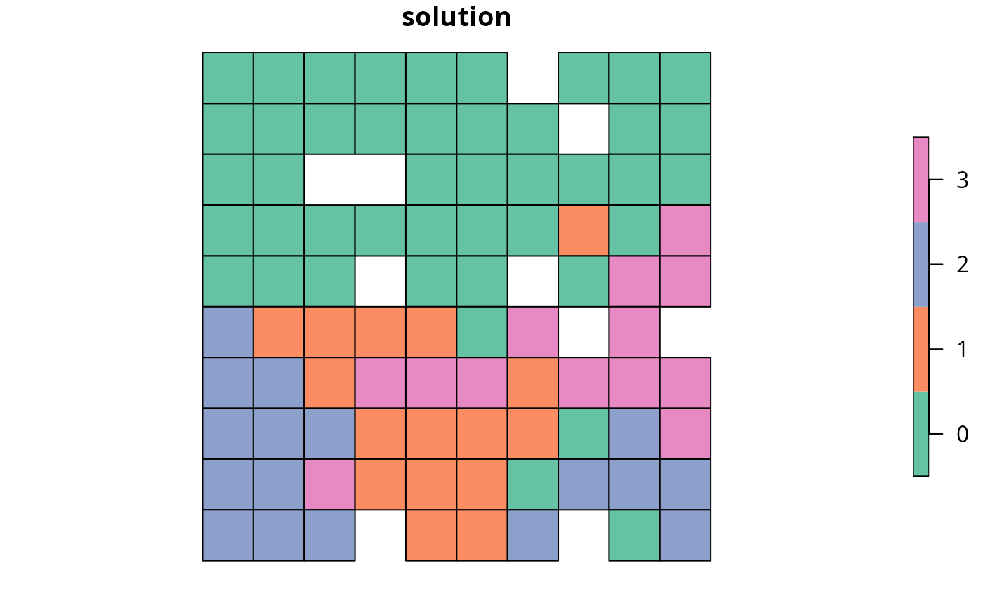
# plot solution
plot(category_layer(s4), main = "solution", axes = FALSE)
# build multi-zone conservation problem with raster data
p4 <-
problem(sim_zones_pu_raster, sim_zones_features) %>%
add_min_set_objective() %>%
add_relative_targets(matrix(runif(15, 0.1, 0.2), nrow = 5, ncol = 3)) %>%
add_binary_decisions() %>%
add_default_solver(verbose = FALSE)
# solve problem
s4 <- solve(p4)
# print solution
print(s4)
#> class : SpatRaster
#> size : 10, 10, 3 (nrow, ncol, nlyr)
#> resolution : 0.1, 0.1 (x, y)
#> extent : 0, 1, 0, 1 (xmin, xmax, ymin, ymax)
#> coord. ref. : WGS 84 / Pseudo-Mercator (EPSG:3857)
#> source(s) : memory
#> varnames : sim_zones_pu_raster
#> sim_zones_pu_raster
#> sim_zones_pu_raster
#> names : zone_1, zone_2, zone_3
#> min values : 0, 0, 0
#> max values : 1, 1, 1
# calculate feature representation in the solution
r4 <- eval_feature_representation_summary(p4, s4)
print(r4)
#> # A tibble: 20 × 5
#> summary feature total_amount absolute_held relative_held
#> <chr> <chr> <dbl> <dbl> <dbl>
#> 1 overall feature_1 250. 43.5 0.174
#> 2 overall feature_2 93.6 16.5 0.176
#> 3 overall feature_3 216. 35.1 0.163
#> 4 overall feature_4 128. 24.0 0.188
#> 5 overall feature_5 170. 30.6 0.180
#> 6 zone_1 feature_1 83.3 16.2 0.195
#> 7 zone_1 feature_2 31.2 5.46 0.175
#> 8 zone_1 feature_3 72.0 13.4 0.186
#> 9 zone_1 feature_4 42.7 7.25 0.170
#> 10 zone_1 feature_5 56.7 11.0 0.194
#> 11 zone_2 feature_1 83.3 14.6 0.175
#> 12 zone_2 feature_2 31.2 4.91 0.157
#> 13 zone_2 feature_3 72.0 10.9 0.152
#> 14 zone_2 feature_4 42.7 8.30 0.194
#> 15 zone_2 feature_5 56.7 10.7 0.188
#> 16 zone_3 feature_1 83.3 12.7 0.152
#> 17 zone_3 feature_2 31.2 6.14 0.197
#> 18 zone_3 feature_3 72.0 10.8 0.150
#> 19 zone_3 feature_4 42.7 8.47 0.199
#> 20 zone_3 feature_5 56.7 8.94 0.158
# plot solution
plot(category_layer(s4), main = "solution", axes = FALSE)
 # build multi-zone conservation problem with polygon data
p5 <-
problem(
sim_zones_pu_polygons, sim_zones_features,
cost_column = c("cost_1", "cost_2", "cost_3")
) %>%
add_min_set_objective() %>%
add_relative_targets(matrix(runif(15, 0.1, 0.2), nrow = 5, ncol = 3)) %>%
add_binary_decisions() %>%
add_default_solver(verbose = FALSE)
# solve problem
s5 <- solve(p5)
# print first six rows of the attribute table
print(head(s5))
#> Simple feature collection with 6 features and 9 fields
#> Geometry type: POLYGON
#> Dimension: XY
#> Bounding box: xmin: 0 ymin: 0.9 xmax: 0.6 ymax: 1
#> Projected CRS: WGS 84 / Pseudo-Mercator
#> # A tibble: 6 × 10
#> cost_1 cost_2 cost_3 locked_1 locked_2 locked_3 solution_1_zone_1
#> <dbl> <dbl> <dbl> <lgl> <lgl> <lgl> <dbl>
#> 1 216. 183. 205. FALSE FALSE FALSE 0
#> 2 213. 189. 210. FALSE FALSE FALSE 0
#> 3 207. 194. 215. TRUE FALSE FALSE 0
#> 4 209. 198. 219. FALSE FALSE FALSE 0
#> 5 214. 200. 221. FALSE FALSE FALSE 0
#> 6 214. 203. 225. FALSE FALSE FALSE 0
#> # ℹ 3 more variables: solution_1_zone_2 <dbl>, solution_1_zone_3 <dbl>,
#> # geometry <POLYGON [m]>
# calculate feature representation in the solution
r5 <- eval_feature_representation_summary(
p5, s5[, c("solution_1_zone_1", "solution_1_zone_2", "solution_1_zone_3")]
)
print(r5)
#> # A tibble: 20 × 5
#> summary feature total_amount absolute_held relative_held
#> <chr> <chr> <dbl> <dbl> <dbl>
#> 1 overall feature_1 225. 40.8 0.181
#> 2 overall feature_2 83.9 13.4 0.160
#> 3 overall feature_3 195. 33.8 0.173
#> 4 overall feature_4 114. 19.0 0.166
#> 5 overall feature_5 154. 28.1 0.183
#> 6 zone_1 feature_1 75.1 14.3 0.190
#> 7 zone_1 feature_2 28.0 5.06 0.181
#> 8 zone_1 feature_3 65.0 12.4 0.191
#> 9 zone_1 feature_4 38.0 6.51 0.171
#> 10 zone_1 feature_5 51.2 9.34 0.183
#> 11 zone_2 feature_1 75.1 15.3 0.204
#> 12 zone_2 feature_2 28.0 4.60 0.164
#> 13 zone_2 feature_3 65.0 12.7 0.196
#> 14 zone_2 feature_4 38.0 6.07 0.160
#> 15 zone_2 feature_5 51.2 10.7 0.209
#> 16 zone_3 feature_1 75.1 11.2 0.149
#> 17 zone_3 feature_2 28.0 3.74 0.134
#> 18 zone_3 feature_3 65.0 8.70 0.134
#> 19 zone_3 feature_4 38.0 6.38 0.168
#> 20 zone_3 feature_5 51.2 8.05 0.157
# create new column representing the zone id that each planning unit
# was allocated to in the solution
s5$solution <- category_vector(
s5[, c("solution_1_zone_1", "solution_1_zone_2", "solution_1_zone_3")]
)
s5$solution <- factor(s5$solution)
# plot solution
plot(s5[, "solution"])
# build multi-zone conservation problem with polygon data
p5 <-
problem(
sim_zones_pu_polygons, sim_zones_features,
cost_column = c("cost_1", "cost_2", "cost_3")
) %>%
add_min_set_objective() %>%
add_relative_targets(matrix(runif(15, 0.1, 0.2), nrow = 5, ncol = 3)) %>%
add_binary_decisions() %>%
add_default_solver(verbose = FALSE)
# solve problem
s5 <- solve(p5)
# print first six rows of the attribute table
print(head(s5))
#> Simple feature collection with 6 features and 9 fields
#> Geometry type: POLYGON
#> Dimension: XY
#> Bounding box: xmin: 0 ymin: 0.9 xmax: 0.6 ymax: 1
#> Projected CRS: WGS 84 / Pseudo-Mercator
#> # A tibble: 6 × 10
#> cost_1 cost_2 cost_3 locked_1 locked_2 locked_3 solution_1_zone_1
#> <dbl> <dbl> <dbl> <lgl> <lgl> <lgl> <dbl>
#> 1 216. 183. 205. FALSE FALSE FALSE 0
#> 2 213. 189. 210. FALSE FALSE FALSE 0
#> 3 207. 194. 215. TRUE FALSE FALSE 0
#> 4 209. 198. 219. FALSE FALSE FALSE 0
#> 5 214. 200. 221. FALSE FALSE FALSE 0
#> 6 214. 203. 225. FALSE FALSE FALSE 0
#> # ℹ 3 more variables: solution_1_zone_2 <dbl>, solution_1_zone_3 <dbl>,
#> # geometry <POLYGON [m]>
# calculate feature representation in the solution
r5 <- eval_feature_representation_summary(
p5, s5[, c("solution_1_zone_1", "solution_1_zone_2", "solution_1_zone_3")]
)
print(r5)
#> # A tibble: 20 × 5
#> summary feature total_amount absolute_held relative_held
#> <chr> <chr> <dbl> <dbl> <dbl>
#> 1 overall feature_1 225. 40.8 0.181
#> 2 overall feature_2 83.9 13.4 0.160
#> 3 overall feature_3 195. 33.8 0.173
#> 4 overall feature_4 114. 19.0 0.166
#> 5 overall feature_5 154. 28.1 0.183
#> 6 zone_1 feature_1 75.1 14.3 0.190
#> 7 zone_1 feature_2 28.0 5.06 0.181
#> 8 zone_1 feature_3 65.0 12.4 0.191
#> 9 zone_1 feature_4 38.0 6.51 0.171
#> 10 zone_1 feature_5 51.2 9.34 0.183
#> 11 zone_2 feature_1 75.1 15.3 0.204
#> 12 zone_2 feature_2 28.0 4.60 0.164
#> 13 zone_2 feature_3 65.0 12.7 0.196
#> 14 zone_2 feature_4 38.0 6.07 0.160
#> 15 zone_2 feature_5 51.2 10.7 0.209
#> 16 zone_3 feature_1 75.1 11.2 0.149
#> 17 zone_3 feature_2 28.0 3.74 0.134
#> 18 zone_3 feature_3 65.0 8.70 0.134
#> 19 zone_3 feature_4 38.0 6.38 0.168
#> 20 zone_3 feature_5 51.2 8.05 0.157
# create new column representing the zone id that each planning unit
# was allocated to in the solution
s5$solution <- category_vector(
s5[, c("solution_1_zone_1", "solution_1_zone_2", "solution_1_zone_3")]
)
s5$solution <- factor(s5$solution)
# plot solution
plot(s5[, "solution"])