Add penalties to a conservation planning problem to account for
symmetric connectivity between planning units.
Symmetric connectivity data describe connectivity information that is not
directional. For example, symmetric connectivity data could describe which
planning units are adjacent to each other (see adjacency_matrix()),
or which planning units are within threshold distance of each other (see
proximity_matrix()).
Usage
# S4 method for class 'ConservationProblem,ANY,ANY,matrix'
add_connectivity_penalties(x, penalty, zones, data)

# S4 method for class 'ConservationProblem,ANY,ANY,Matrix'
add_connectivity_penalties(x, penalty, zones, data)

# S4 method for class 'ConservationProblem,ANY,ANY,data.frame'
add_connectivity_penalties(x, penalty, zones, data)

# S4 method for class 'ConservationProblem,ANY,ANY,dgCMatrix'
add_connectivity_penalties(x, penalty, zones, data)

# S4 method for class 'ConservationProblem,ANY,ANY,array'
add_connectivity_penalties(x, penalty, zones, data)
Arguments
- x
problem()object.- penalty
numericvalue denoting the importance of selecting planning units with strong connectivity between them compared to the main problem objective (e.g., solution cost ifxhas a minimum set objective set usingadd_min_set_objective()). Higherpenaltyvalues can be used to obtain solutions with a high degree of connectivity, and smallerpenaltyvalues can be used to obtain solutions with a small degree of connectivity. Note that negativepenaltyvalues can be used to obtain solutions that avoid connectivity.- zones
matrixorMatrixobject describing the level of connectivity between different zones. Each row and column corresponds to a different zone inx, and cell values indicate the level of connectivity between each combination of zones. Cell values along the diagonal of the matrix represent the level of connectivity between planning units allocated to the same zone. Cell values must range between 1 and -1, where negative values favor solutions with weak connectivity. Defaults to an identity matrix (i.e., a matrix with ones along the matrix diagonal and zeros elsewhere), so that planning units are only considered to be connected when they are allocated to the same zone. Note thatzonesis only required when working with multiple zones anddatais amatrixorMatrixobject. Ifdatais anarrayordata.framewith data for multiple zones (e.g., using the"zone1"and"zone2"column names), thenzonesmust beNULL.- data
matrix,Matrix,data.frame, orarrayobject containing connectivity data. The connectivity values correspond to the strength of connectivity between different planning units. Thus connections between planning units that are associated with higher values are more favorable in the solution. See the Data format section for more information.
Value
An updated problem() object with the penalties added to it.
Details
This function adds penalties to conservation planning problem to penalize solutions that have low connectivity. Specifically, it favors pair-wise connections between planning units that have high connectivity values (based on Önal and Briers 2002).
Data format
The following formats can be used to specify data.
dataas amatrix/MatrixobjectHere rows and columns correspond to different planning units and cell values denote the strength of connectivity between two planning units. Cells that occur along the matrix diagonal are treated as weights which indicate that planning units are more desirable in the solution. With this format,
zonescan be used to control the strength of connectivity between planning units in different zones. Note that the default forzonesis to treat planning units allocated to different zones as having zero connectivity.dataas adata.frameobjectHere rows correspond to a pair of planning units and columns provide information about each pair of planning units. In particular,
datamust have the columns:"id1","id2", and"boundary". The"id1"and"id2"columns contain identifiers (indices) for a pair of planning units, and the"boundary"column contains the strength of connectivity between them (following the Marxan format). Ifxhas multiple zones, then the"zone1"and"zone2"columns can optionally be provided to manually specify the connectivity values between planning units when they are allocated to particular zones. Note that if the"zone1"and"zone2"columns are present, thenzonesmust beNULL.dataas anarrayobjectHere a four-dimension array is used to specify connectivity data, where cell values indicate the strength of connectivity between planning units when they are assigned to specific management zones. The first two dimensions (i.e., rows and columns) indicate the strength of connectivity between different planning units and the second two dimensions indicate the different management zones. Thus the
data[1, 2, 3, 4]indicates the strength of connectivity between planning unit 1 and planning unit 2 when planning unit 1 is assigned to zone 3 and planning unit 2 is assigned to zone 4.
Mathematical formulation
The connectivity penalties are implemented using the following equations.
Let \(I\) represent the set of planning units
(indexed by \(i\) or \(j\)), \(Z\) represent the set
of management zones (indexed by \(z\) or \(y\)), and \(X_{iz}\)
represent the decision variable for planning unit \(i\) for in zone
\(z\) (e.g., with binary
values one indicating if planning unit is allocated or not). Also, let
\(p\) represent penalty, \(D\) represent
data, and \(W\) represent zones.
If data is specified as a matrix or
Matrix object, then the penalties are calculated as:
$$ \sum_{i}^{I} \sum_{j}^{I} \sum_{z}^{Z} \sum_{y}^{Z} (-p \times X_{iz} \times X_{jy} \times D_{ij} \times W_{zy})$$
Otherwise, if data is specified as a
data.frame or array object, then the penalties are
calculated as:
$$ \sum_{i}^{I} \sum_{j}^{I} \sum_{z}^{Z} \sum_{y}^{Z} (-p \times X_{iz} \times X_{jy} \times D_{ijzy})$$
Note that when the problem objective is to maximize some measure of benefit and not minimize some measure of cost, the term \(-p\) is replaced with \(p\). Additionally, to linearize the problem, the expression \(X_{iz} \times X_{jy}\) is modeled using a set of continuous variables (bounded between 0 and 1) based on Beyer et al. (2016).
Notes
In previous versions, this function aimed to handle both symmetric and
asymmetric connectivity data. This meant that the mathematical
formulation used to account for asymmetric connectivity was different
to that implemented by the Marxan software
(see Beger et al. for details). To ensure that asymmetric connectivity is
handled in a similar manner to the Marxan software, the
add_asym_connectivity_penalties() function should now be used for
asymmetric connectivity data.
References
Beger M, Linke S, Watts M, Game E, Treml E, Ball I, and Possingham, HP (2010) Incorporating asymmetric connectivity into spatial decision making for conservation, Conservation Letters, 3: 359–368.
Beyer HL, Dujardin Y, Watts ME, and Possingham HP (2016) Solving conservation planning problems with integer linear programming. Ecological Modelling, 228: 14–22.
Önal H, and Briers RA (2002) Incorporating spatial criteria in optimum reserve network selection. Proceedings of the Royal Society of London. Series B: Biological Sciences, 269: 2437–2441.
See also
See penalties for an overview of all functions for adding penalties.
Also see add_asym_connectivity_penalties() to account for
asymmetric connectivity between planning units.
Additionally, see calibrate_cohon_penalty() for assistance with selecting
an appropriate penalty value.
Other functions for adding penalties:
add_asym_connectivity_penalties(),
add_boundary_penalties(),
add_cost_penalties(),
add_feature_weights(),
add_linear_penalties(),
add_neighbor_penalties()
Examples
# set seed for reproducibility
set.seed(600)
# load data
sim_pu_polygons <- get_sim_pu_polygons()
sim_features <- get_sim_features()
sim_zones_pu_raster <- get_sim_zones_pu_raster()
sim_zones_features <- get_sim_zones_features()
# create basic problem
p1 <-
problem(sim_pu_polygons, sim_features, "cost") %>%
add_min_set_objective() %>%
add_relative_targets(0.2) %>%
add_default_solver(verbose = FALSE)
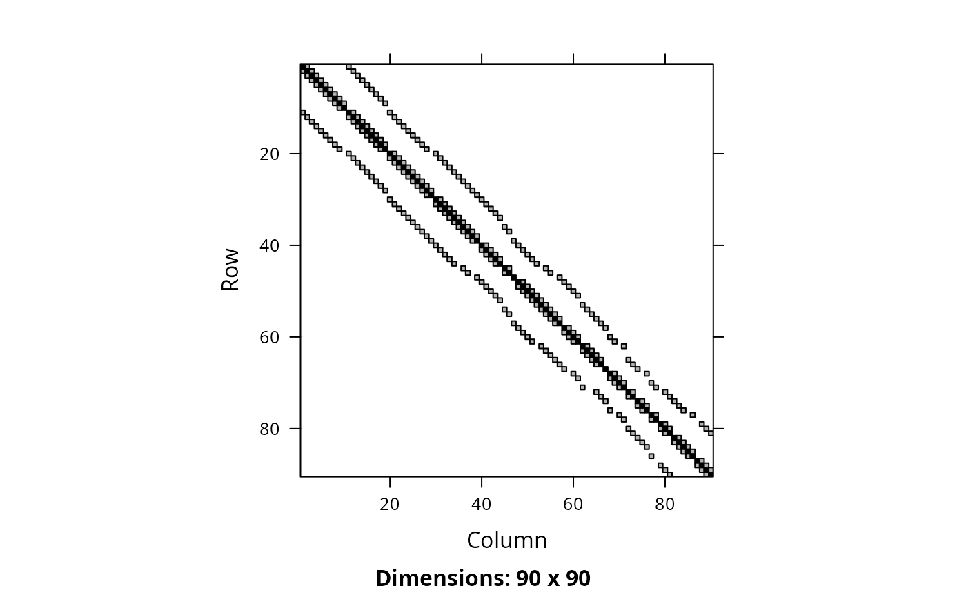
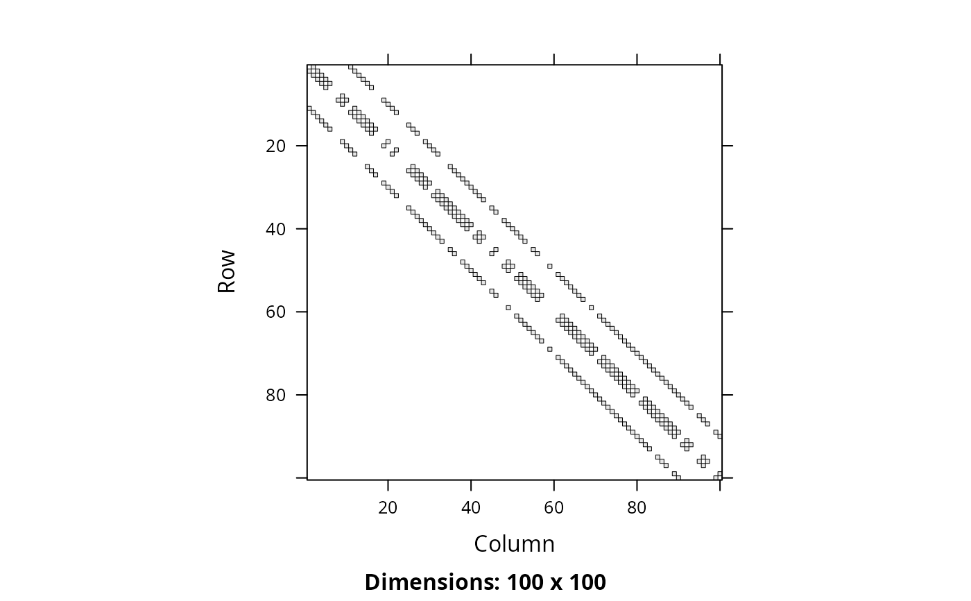
# create a symmetric connectivity matrix where the connectivity between
# two planning units corresponds to their shared boundary length
b_matrix <- boundary_matrix(sim_pu_polygons)
# rescale matrix values to have a maximum value of 1
b_matrix <- rescale_matrix(b_matrix, max = 1)
# visualize connectivity matrix
Matrix::image(b_matrix)
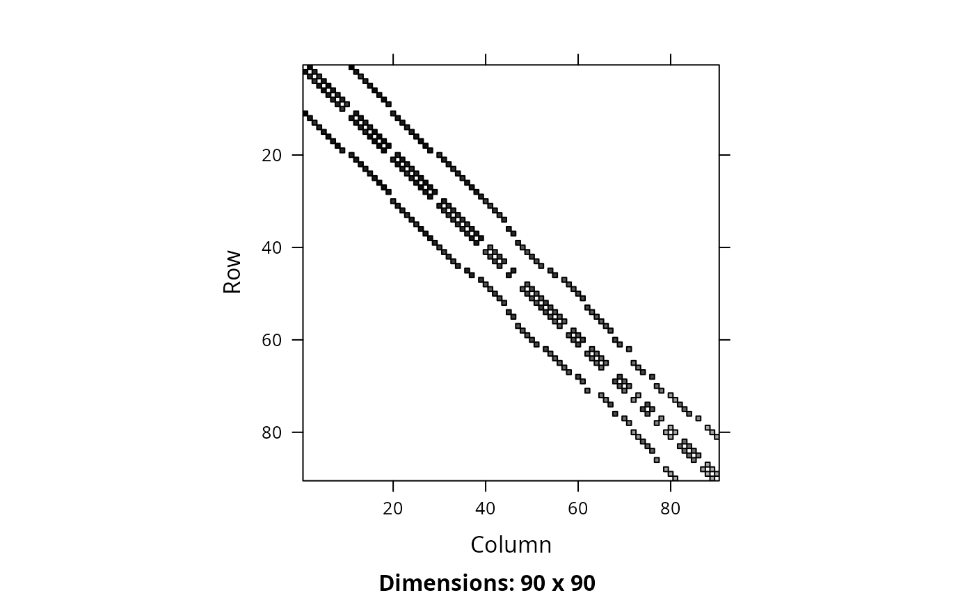
 # create a symmetric connectivity matrix where the connectivity between
# two planning units corresponds to their spatial proximity
# i.e., planning units that are further apart share less connectivity
centroids <- sf::st_coordinates(
suppressWarnings(sf::st_centroid(sim_pu_polygons))
)
d_matrix <- (1 / (Matrix::Matrix(as.matrix(dist(centroids))) + 1))
# rescale matrix values to have a maximum value of 1
d_matrix <- rescale_matrix(d_matrix, max = 1)
# remove connections between planning units with values below a threshold to
# reduce run-time
d_matrix[d_matrix < 0.8] <- 0
# visualize connectivity matrix
Matrix::image(d_matrix)
# create a symmetric connectivity matrix where the connectivity between
# two planning units corresponds to their spatial proximity
# i.e., planning units that are further apart share less connectivity
centroids <- sf::st_coordinates(
suppressWarnings(sf::st_centroid(sim_pu_polygons))
)
d_matrix <- (1 / (Matrix::Matrix(as.matrix(dist(centroids))) + 1))
# rescale matrix values to have a maximum value of 1
d_matrix <- rescale_matrix(d_matrix, max = 1)
# remove connections between planning units with values below a threshold to
# reduce run-time
d_matrix[d_matrix < 0.8] <- 0
# visualize connectivity matrix
Matrix::image(d_matrix)
 # create a symmetric connectivity matrix where the connectivity
# between adjacent two planning units corresponds to their combined
# value in a column of the planning unit data
# for example, this column could describe the extent of native vegetation in
# each planning unit and we could use connectivity penalties to identify
# solutions that cluster planning units together that both contain large
# amounts of native vegetation
c_matrix <- connectivity_matrix(sim_pu_polygons, "cost")
# rescale matrix values to have a maximum value of 1
c_matrix <- rescale_matrix(c_matrix, max = 1)
# visualize connectivity matrix
Matrix::image(c_matrix)
# create a symmetric connectivity matrix where the connectivity
# between adjacent two planning units corresponds to their combined
# value in a column of the planning unit data
# for example, this column could describe the extent of native vegetation in
# each planning unit and we could use connectivity penalties to identify
# solutions that cluster planning units together that both contain large
# amounts of native vegetation
c_matrix <- connectivity_matrix(sim_pu_polygons, "cost")
# rescale matrix values to have a maximum value of 1
c_matrix <- rescale_matrix(c_matrix, max = 1)
# visualize connectivity matrix
Matrix::image(c_matrix)
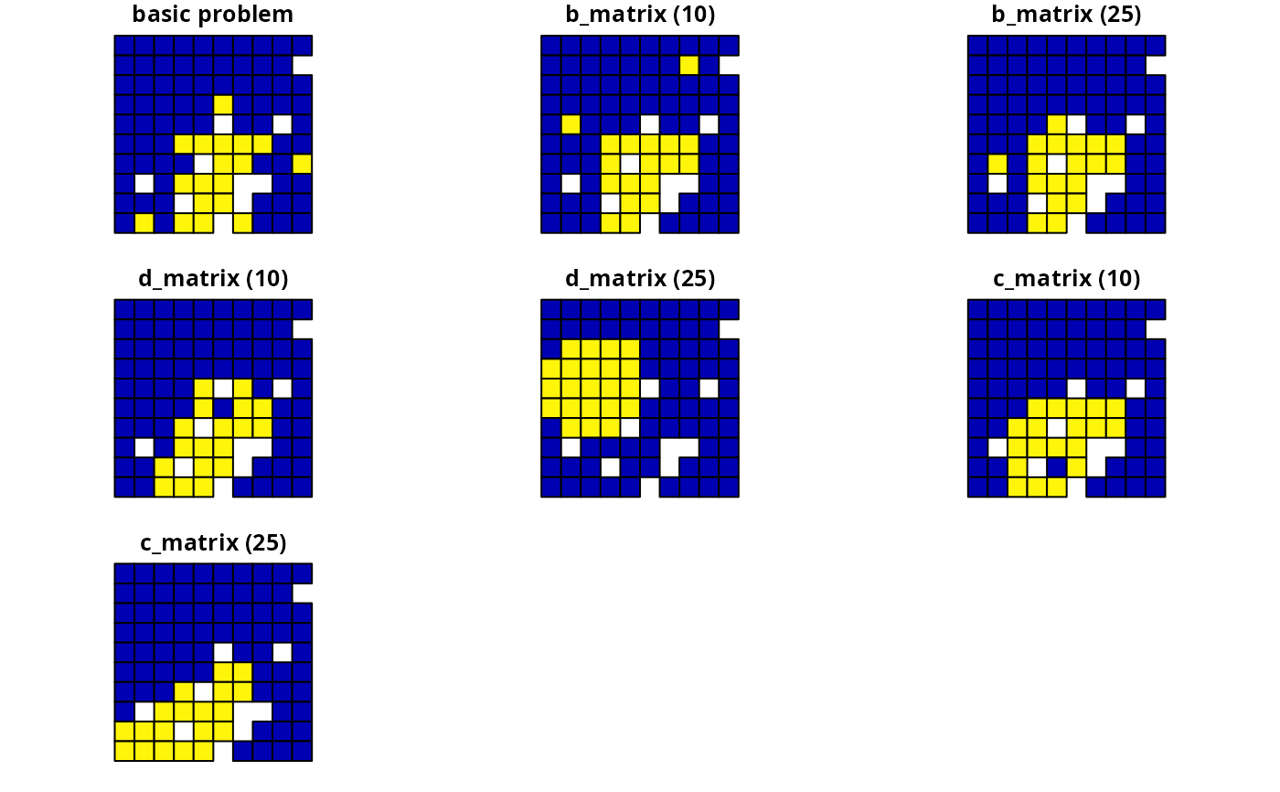
 # create penalties
penalties <- c(10, 25)
# create problems using the different connectivity matrices and penalties
p2 <- list(
p1,
p1 %>% add_connectivity_penalties(penalties[1], data = b_matrix),
p1 %>% add_connectivity_penalties(penalties[2], data = b_matrix),
p1 %>% add_connectivity_penalties(penalties[1], data = d_matrix),
p1 %>% add_connectivity_penalties(penalties[2], data = d_matrix),
p1 %>% add_connectivity_penalties(penalties[1], data = c_matrix),
p1 %>% add_connectivity_penalties(penalties[2], data = c_matrix)
)
# solve problems
s2 <- lapply(p2, solve)
# create single object with all solutions
s2 <- sf::st_sf(
tibble::tibble(
p2_1 = s2[[1]]$solution_1,
p2_2 = s2[[2]]$solution_1,
p2_3 = s2[[3]]$solution_1,
p2_4 = s2[[4]]$solution_1,
p2_5 = s2[[5]]$solution_1,
p2_6 = s2[[6]]$solution_1,
p2_7 = s2[[7]]$solution_1
),
geometry = sf::st_geometry(s2[[1]])
)
names(s2)[1:7] <- c(
"basic problem",
paste0("b_matrix (", penalties,")"),
paste0("d_matrix (", penalties,")"),
paste0("c_matrix (", penalties,")")
)
# plot solutions
plot(s2)
# create penalties
penalties <- c(10, 25)
# create problems using the different connectivity matrices and penalties
p2 <- list(
p1,
p1 %>% add_connectivity_penalties(penalties[1], data = b_matrix),
p1 %>% add_connectivity_penalties(penalties[2], data = b_matrix),
p1 %>% add_connectivity_penalties(penalties[1], data = d_matrix),
p1 %>% add_connectivity_penalties(penalties[2], data = d_matrix),
p1 %>% add_connectivity_penalties(penalties[1], data = c_matrix),
p1 %>% add_connectivity_penalties(penalties[2], data = c_matrix)
)
# solve problems
s2 <- lapply(p2, solve)
# create single object with all solutions
s2 <- sf::st_sf(
tibble::tibble(
p2_1 = s2[[1]]$solution_1,
p2_2 = s2[[2]]$solution_1,
p2_3 = s2[[3]]$solution_1,
p2_4 = s2[[4]]$solution_1,
p2_5 = s2[[5]]$solution_1,
p2_6 = s2[[6]]$solution_1,
p2_7 = s2[[7]]$solution_1
),
geometry = sf::st_geometry(s2[[1]])
)
names(s2)[1:7] <- c(
"basic problem",
paste0("b_matrix (", penalties,")"),
paste0("d_matrix (", penalties,")"),
paste0("c_matrix (", penalties,")")
)
# plot solutions
plot(s2)
 # create minimal multi-zone problem and limit solver to one minute
# to obtain solutions in a short period of time
p3 <-
problem(sim_zones_pu_raster, sim_zones_features) %>%
add_min_set_objective() %>%
add_relative_targets(matrix(0.15, nrow = 5, ncol = 3)) %>%
add_binary_decisions() %>%
add_default_solver(time_limit = 60, verbose = FALSE)
# create matrix showing which planning units are adjacent to other units
a_matrix <- adjacency_matrix(sim_zones_pu_raster)
# visualize matrix
Matrix::image(a_matrix)
# create minimal multi-zone problem and limit solver to one minute
# to obtain solutions in a short period of time
p3 <-
problem(sim_zones_pu_raster, sim_zones_features) %>%
add_min_set_objective() %>%
add_relative_targets(matrix(0.15, nrow = 5, ncol = 3)) %>%
add_binary_decisions() %>%
add_default_solver(time_limit = 60, verbose = FALSE)
# create matrix showing which planning units are adjacent to other units
a_matrix <- adjacency_matrix(sim_zones_pu_raster)
# visualize matrix
Matrix::image(a_matrix)
 # create a zone matrix where connectivities are only present between
# planning units that are allocated to the same zone
zm1 <- as(diag(3), "Matrix")
# print zone matrix
print(zm1)
#> 3 x 3 diagonal matrix of class "ddiMatrix"
#> [,1] [,2] [,3]
#> [1,] 1 . .
#> [2,] . 1 .
#> [3,] . . 1
# create a zone matrix where connectivities are strongest between
# planning units allocated to different zones
zm2 <- matrix(1, ncol = 3, nrow = 3)
diag(zm2) <- 0
zm2 <- as(zm2, "Matrix")
# print zone matrix
print(zm2)
#> 3 x 3 Matrix of class "dsyMatrix"
#> [,1] [,2] [,3]
#> [1,] 0 1 1
#> [2,] 1 0 1
#> [3,] 1 1 0
# create a zone matrix that indicates that connectivities between planning
# units assigned to the same zone are much higher than connectivities
# assigned to different zones
zm3 <- matrix(0.1, ncol = 3, nrow = 3)
diag(zm3) <- 1
zm3 <- as(zm3, "Matrix")
# print zone matrix
print(zm3)
#> 3 x 3 Matrix of class "dsyMatrix"
#> [,1] [,2] [,3]
#> [1,] 1.0 0.1 0.1
#> [2,] 0.1 1.0 0.1
#> [3,] 0.1 0.1 1.0
# create a zone matrix that indicates that connectivities between planning
# units allocated to zone 1 are very high, connectivities between planning
# units allocated to zones 1 and 2 are moderately high, and connectivities
# planning units allocated to other zones are low
zm4 <- matrix(0.1, ncol = 3, nrow = 3)
zm4[1, 1] <- 1
zm4[1, 2] <- 0.5
zm4[2, 1] <- 0.5
zm4 <- as(zm4, "Matrix")
# print zone matrix
print(zm4)
#> 3 x 3 Matrix of class "dsyMatrix"
#> [,1] [,2] [,3]
#> [1,] 1.0 0.5 0.1
#> [2,] 0.5 0.1 0.1
#> [3,] 0.1 0.1 0.1
# create a zone matrix with strong connectivities between planning units
# allocated to the same zone, moderate connectivities between planning
# unit allocated to zone 1 and zone 2, and negative connectivities between
# planning units allocated to zone 3 and the other two zones
zm5 <- matrix(-1, ncol = 3, nrow = 3)
zm5[1, 2] <- 0.5
zm5[2, 1] <- 0.5
diag(zm5) <- 1
zm5 <- as(zm5, "Matrix")
# print zone matrix
print(zm5)
#> 3 x 3 Matrix of class "dsyMatrix"
#> [,1] [,2] [,3]
#> [1,] 1.0 0.5 -1
#> [2,] 0.5 1.0 -1
#> [3,] -1.0 -1.0 1
# create vector of penalties to use creating problems
penalties2 <- c(5, 15)
# create multi-zone problems using the adjacent connectivity matrix and
# different zone matrices
p4 <- list(
p3,
p3 %>% add_connectivity_penalties(penalties2[1], zm1, a_matrix),
p3 %>% add_connectivity_penalties(penalties2[2], zm1, a_matrix),
p3 %>% add_connectivity_penalties(penalties2[1], zm2, a_matrix),
p3 %>% add_connectivity_penalties(penalties2[2], zm2, a_matrix),
p3 %>% add_connectivity_penalties(penalties2[1], zm3, a_matrix),
p3 %>% add_connectivity_penalties(penalties2[2], zm3, a_matrix),
p3 %>% add_connectivity_penalties(penalties2[1], zm4, a_matrix),
p3 %>% add_connectivity_penalties(penalties2[2], zm4, a_matrix),
p3 %>% add_connectivity_penalties(penalties2[1], zm5, a_matrix),
p3 %>% add_connectivity_penalties(penalties2[2], zm5, a_matrix)
)
# solve problems
s4 <- lapply(p4, solve)
s4 <- lapply(s4, category_layer)
s4 <- terra::rast(s4)
names(s4) <- c(
"basic problem",
paste0("zm", rep(seq_len(5), each = 2), " (", rep(penalties2, 2), ")")
)
# plot solutions
plot(s4, axes = FALSE)
# create a zone matrix where connectivities are only present between
# planning units that are allocated to the same zone
zm1 <- as(diag(3), "Matrix")
# print zone matrix
print(zm1)
#> 3 x 3 diagonal matrix of class "ddiMatrix"
#> [,1] [,2] [,3]
#> [1,] 1 . .
#> [2,] . 1 .
#> [3,] . . 1
# create a zone matrix where connectivities are strongest between
# planning units allocated to different zones
zm2 <- matrix(1, ncol = 3, nrow = 3)
diag(zm2) <- 0
zm2 <- as(zm2, "Matrix")
# print zone matrix
print(zm2)
#> 3 x 3 Matrix of class "dsyMatrix"
#> [,1] [,2] [,3]
#> [1,] 0 1 1
#> [2,] 1 0 1
#> [3,] 1 1 0
# create a zone matrix that indicates that connectivities between planning
# units assigned to the same zone are much higher than connectivities
# assigned to different zones
zm3 <- matrix(0.1, ncol = 3, nrow = 3)
diag(zm3) <- 1
zm3 <- as(zm3, "Matrix")
# print zone matrix
print(zm3)
#> 3 x 3 Matrix of class "dsyMatrix"
#> [,1] [,2] [,3]
#> [1,] 1.0 0.1 0.1
#> [2,] 0.1 1.0 0.1
#> [3,] 0.1 0.1 1.0
# create a zone matrix that indicates that connectivities between planning
# units allocated to zone 1 are very high, connectivities between planning
# units allocated to zones 1 and 2 are moderately high, and connectivities
# planning units allocated to other zones are low
zm4 <- matrix(0.1, ncol = 3, nrow = 3)
zm4[1, 1] <- 1
zm4[1, 2] <- 0.5
zm4[2, 1] <- 0.5
zm4 <- as(zm4, "Matrix")
# print zone matrix
print(zm4)
#> 3 x 3 Matrix of class "dsyMatrix"
#> [,1] [,2] [,3]
#> [1,] 1.0 0.5 0.1
#> [2,] 0.5 0.1 0.1
#> [3,] 0.1 0.1 0.1
# create a zone matrix with strong connectivities between planning units
# allocated to the same zone, moderate connectivities between planning
# unit allocated to zone 1 and zone 2, and negative connectivities between
# planning units allocated to zone 3 and the other two zones
zm5 <- matrix(-1, ncol = 3, nrow = 3)
zm5[1, 2] <- 0.5
zm5[2, 1] <- 0.5
diag(zm5) <- 1
zm5 <- as(zm5, "Matrix")
# print zone matrix
print(zm5)
#> 3 x 3 Matrix of class "dsyMatrix"
#> [,1] [,2] [,3]
#> [1,] 1.0 0.5 -1
#> [2,] 0.5 1.0 -1
#> [3,] -1.0 -1.0 1
# create vector of penalties to use creating problems
penalties2 <- c(5, 15)
# create multi-zone problems using the adjacent connectivity matrix and
# different zone matrices
p4 <- list(
p3,
p3 %>% add_connectivity_penalties(penalties2[1], zm1, a_matrix),
p3 %>% add_connectivity_penalties(penalties2[2], zm1, a_matrix),
p3 %>% add_connectivity_penalties(penalties2[1], zm2, a_matrix),
p3 %>% add_connectivity_penalties(penalties2[2], zm2, a_matrix),
p3 %>% add_connectivity_penalties(penalties2[1], zm3, a_matrix),
p3 %>% add_connectivity_penalties(penalties2[2], zm3, a_matrix),
p3 %>% add_connectivity_penalties(penalties2[1], zm4, a_matrix),
p3 %>% add_connectivity_penalties(penalties2[2], zm4, a_matrix),
p3 %>% add_connectivity_penalties(penalties2[1], zm5, a_matrix),
p3 %>% add_connectivity_penalties(penalties2[2], zm5, a_matrix)
)
# solve problems
s4 <- lapply(p4, solve)
s4 <- lapply(s4, category_layer)
s4 <- terra::rast(s4)
names(s4) <- c(
"basic problem",
paste0("zm", rep(seq_len(5), each = 2), " (", rep(penalties2, 2), ")")
)
# plot solutions
plot(s4, axes = FALSE)
 # create an array to manually specify the connectivities between
# each planning unit when they are allocated to each different zone
# for real-world problems, these connectivities would be generated using
# data - but here these connectivity values are assigned as random
# ones or zeros
c_array <- array(0, c(rep(ncell(sim_zones_pu_raster[[1]]), 2), 3, 3))
for (z1 in seq_len(3))
for (z2 in seq_len(3))
c_array[, , z1, z2] <- round(
runif(ncell(sim_zones_pu_raster[[1]]) ^ 2, 0, 0.505)
)
# create a problem with the manually specified connectivity array
# note that the zones is set to NULL because the connectivity
# data is an array
p5 <- list(
p3,
p3 %>% add_connectivity_penalties(15, zones = NULL, c_array)
)
# solve problems
s5 <- lapply(p5, solve)
s5 <- lapply(s5, category_layer)
s5 <- terra::rast(s5)
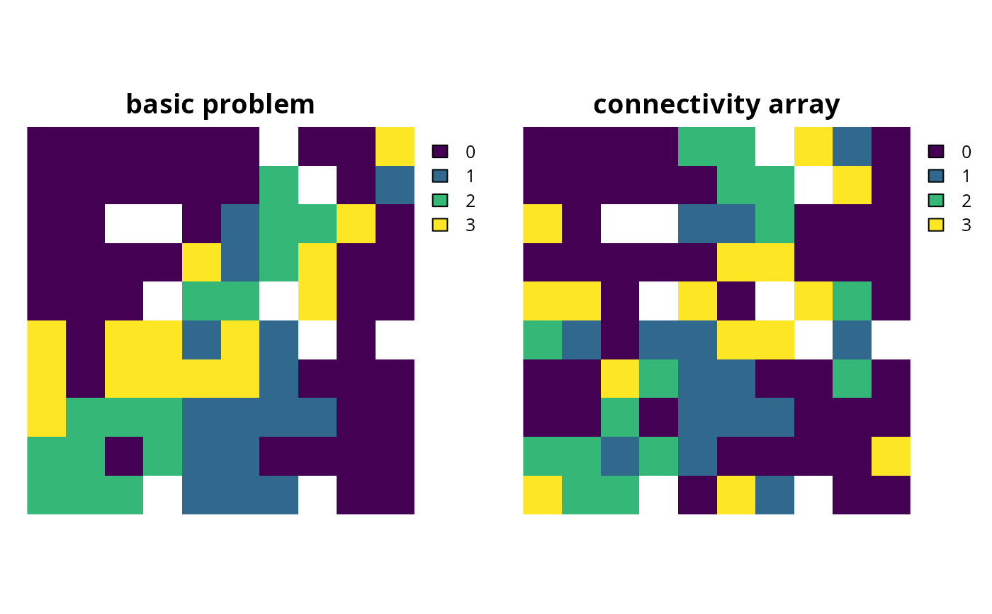
names(s5) <- c("basic problem", "connectivity array")
# plot solutions
plot(s5, axes = FALSE)
# create an array to manually specify the connectivities between
# each planning unit when they are allocated to each different zone
# for real-world problems, these connectivities would be generated using
# data - but here these connectivity values are assigned as random
# ones or zeros
c_array <- array(0, c(rep(ncell(sim_zones_pu_raster[[1]]), 2), 3, 3))
for (z1 in seq_len(3))
for (z2 in seq_len(3))
c_array[, , z1, z2] <- round(
runif(ncell(sim_zones_pu_raster[[1]]) ^ 2, 0, 0.505)
)
# create a problem with the manually specified connectivity array
# note that the zones is set to NULL because the connectivity
# data is an array
p5 <- list(
p3,
p3 %>% add_connectivity_penalties(15, zones = NULL, c_array)
)
# solve problems
s5 <- lapply(p5, solve)
s5 <- lapply(s5, category_layer)
s5 <- terra::rast(s5)
names(s5) <- c("basic problem", "connectivity array")
# plot solutions
plot(s5, axes = FALSE)