Evaluate solution importance using replacement cost scores

Calculate importance scores for planning units selected in a solution based on the replacement cost method (Cabeza and Moilanen 2006).

Usage

eval_replacement_importance(
  x,
  solution,
  rescale = TRUE,
  run_checks = TRUE,
  force = FALSE,
  threads = 1L
)

Arguments

x: problem() object.
solution: numeric, matrix, data.frame, terra::rast(), or sf::sf() object. Note that solution must have the same format as the planning unit data in x. See the Solution format section for more information.
rescale: logical flag indicating if replacement cost values – excepting infinite (Inf) and zero values – should be rescaled to range between 0.01 and 1. Defaults to TRUE.
run_checks: logical flag indicating whether presolve checks should be run prior solving the problem. These checks are performed using the presolve_check() function. Defaults to TRUE. Skipping these checks may reduce run time for large problems.
force: logical flag indicating if an attempt should be made to solve the problem even if potential issues were detected during the presolve checks. Defaults to FALSE.
threads: integer value denoting the number of threads to use during optimization. Broadly speaking, we recommend setting threads to be no higher than the number of computational cores minus one or two (e.g., threads = parallel::detectCores(TRUE) - 2). This is because setting threads to be equal to the number of computational cores means that the solver and is fighting for resources with other software (e.g., Dropbox, iCloud, OneDrive, software updates, antivirus software, internet browsers) and, in turn, can result in computational bottlenecks that slow run times. Additionally, when setting threads to be a value greater than 1, we recommend checking memory (RAM) usage during the optimization process to ensure that the solver does not use up the majority of available memory. This is because solving optimization problems with multiple threads can involve creating multiple copies of the problem (e.g., threads = 5 may mean 5 copies) and exhausting most of the available memory will drastically slow run times. Defaults to 1.

Value

A numeric, matrix, data.frame, terra::rast(), or sf::sf() object containing the importance scores for each planning unit in the solution. Specifically, the returned object is in the same format as the planning unit data in x.

Details

This function implements a modified version of the replacement cost method (Cabeza and Moilanen 2006). Specifically, the score for each planning unit is calculated as the difference in the objective value of a solution when each planning unit is locked out and the optimization processes rerun with all other selected planning units locked in. In other words, the replacement cost metric corresponds to change in solution quality incurred if a given planning unit cannot be acquired when implementing the solution and the next best planning unit (or set of planning units) will need to be considered instead. Thus planning units with a higher score are more important (and irreplaceable). For example, when using the minimum set objective function (add_min_set_objective()), the replacement cost scores correspond to the additional costs needed to meet targets when each planning unit is locked out. When using the maximum weighted sum objective (add_max_wtd_sum_objective(), the replacement cost scores correspond to the reduction in the weighted sum scores when each planning unit is locked out. Infinite values mean that no feasible solution exists when planning units are locked out—they are absolutely essential for obtaining a solution (e.g., they contain rare species that are not found in any other planning units or were locked in). Zeros values mean that planning units can be swapped with other planning units and this will have no effect on the performance of the solution at all (e.g., because they were only selected due to spatial fragmentation penalties).

These calculations can take a long time to complete for large or complex conservation planning problems. As such, we recommend using this method for small or moderate-sized conservation planning problems (e.g., < 30,000 planning units). To reduce run time, we recommend calculating these scores without additional penalties (e.g., add_boundary_penalties()) or spatial constraints (e.g., add_contiguity_constraints()). To further reduce run time, we recommend using proportion-type decisions when calculating the scores (see below for an example).

Solution format

Broadly speaking, solution must be in the same format as the planning unit data in x. Further details on the correct format are listed separately for each of the different planning unit data formats.

x has numeric planning units: Here solution must be a numeric vector with each element corresponding to a different planning unit. It should have the same number of planning units as those in x. Additionally, any planning units with missing cost (NA) values should also have missing (NA) values in the solution.
x has matrix planning units: Here solution must be a matrix vector with each row corresponding to a different planning unit, and each column correspond to a different management zone. It should have the same number of planning units and zones as those in x. Additionally, any planning units with missing cost (NA) values for a particular zone should also have a missing (NA) values in solution.
x has terra::rast() planning units: Here solution be a terra::rast() object where different cells correspond to different planning units and layers correspond to a different management zones. It should have the same dimensionality (rows, columns, layers), resolution, extent, and coordinate reference system as the planning units in x. Additionally, any planning units with missing cost (NA) values for a particular zone should also have missing (NA) values in solution.
x has data.frame planning units: Here solution must be a data.frame with each column corresponding to a different zone, each row corresponding to a different planning unit, and cell values corresponding to the solution value. This means that if a data.frame object containing the solution also contains additional columns, then these columns will need to be subsetted prior to using this function (see below for example with sf::sf() data). Additionally, any planning units with missing cost (NA) values for a particular zone should also have missing (NA) values in solution.
x has sf::sf() planning units: Here solution must be a sf::sf() object with each column corresponding to a different zone, each row corresponding to a different planning unit, and cell values corresponding to the solution value. This means that if the sf::sf() object containing the solution also contains additional columns, then these columns will need to be subsetted prior to using this function (see below for example). Additionally, solution must also have the same coordinate reference system as the planning unit data. Furthermore, any planning units with missing cost (NA) values for a particular zone should also have missing (NA) values in solution.

References

Cabeza M and Moilanen A (2006) Replacement cost: A practical measure of site value for cost-effective reserve planning. Biological Conservation, 132: 336–342.

Examples

# set seed for reproducibility
set.seed(600)

# load data
sim_pu_raster <- get_sim_pu_raster()
sim_pu_polygons <- get_sim_pu_polygons()
sim_features <- get_sim_features()
sim_zones_pu_raster <- get_sim_zones_pu_raster()
sim_zones_features <- get_sim_zones_features()

# create minimal problem with binary decisions
p1 <-
  problem(sim_pu_raster, sim_features) %>%
  add_min_set_objective() %>%
  add_relative_targets(0.1) %>%
  add_binary_decisions() %>%
  add_default_solver(gap = 0, verbose = FALSE)

# solve problem
s1 <- solve(p1)

# print solution
print(s1)
#> class       : SpatRaster
#> size        : 10, 10, 1  (nrow, ncol, nlyr)
#> resolution  : 0.1, 0.1  (x, y)
#> extent      : 0, 1, 0, 1  (xmin, xmax, ymin, ymax)
#> coord. ref. : WGS 84 / Pseudo-Mercator (EPSG:3857)
#> source(s)   : memory
#> varname     : sim_pu_raster
#> name        : layer
#> min value   :     0
#> max value   :     1

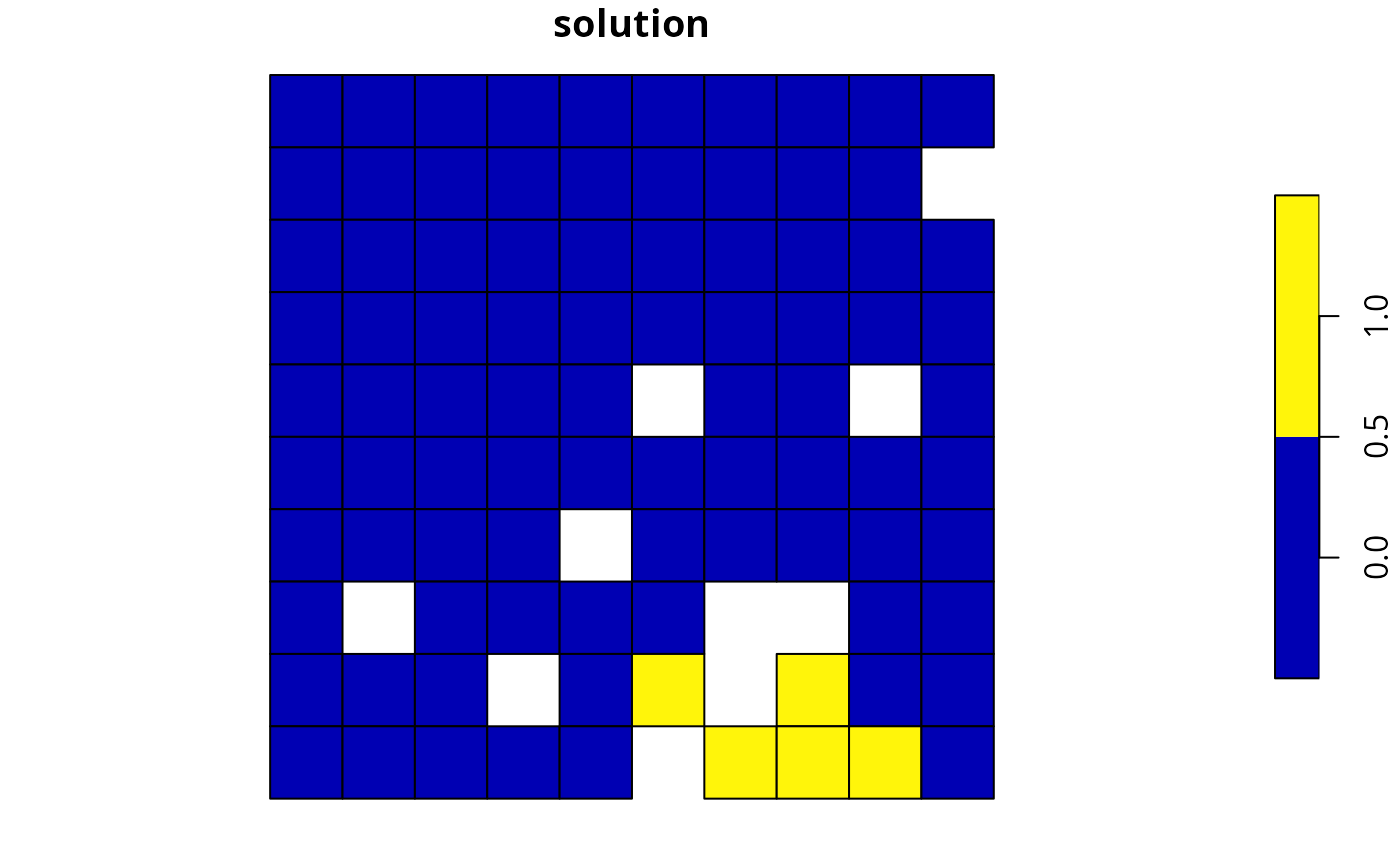
# plot solution
plot(s1, main = "solution", axes = FALSE)


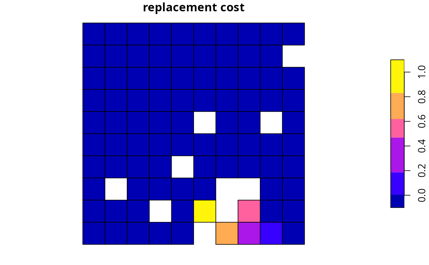
# calculate importance scores
rc1 <- eval_replacement_importance(p1, s1)

# print importance scores
print(rc1)
#> class       : SpatRaster
#> size        : 10, 10, 1  (nrow, ncol, nlyr)
#> resolution  : 0.1, 0.1  (x, y)
#> extent      : 0, 1, 0, 1  (xmin, xmax, ymin, ymax)
#> coord. ref. : WGS 84 / Pseudo-Mercator (EPSG:3857)
#> source(s)   : memory
#> varname     : sim_pu_raster
#> name        : rc
#> min value   :  0
#> max value   :  1

# plot importance scores
plot(rc1, main = "replacement cost", axes = FALSE)


# since replacement cost scores can take a long time to calculate with
# binary decisions, we can calculate them using proportion-type
# decision variables. Note we are still calculating the scores for our
# previous solution (s1), we are just using a different optimization
# problem when calculating the scores.
p2 <-
  problem(sim_pu_raster, sim_features) %>%
  add_min_set_objective() %>%
  add_relative_targets(0.1) %>%
  add_proportion_decisions() %>%
  add_default_solver(gap = 0, verbose = FALSE)

# calculate importance scores using proportion type decisions
rc2 <- eval_replacement_importance(p2, s1)

# print importance scores based on proportion type decisions
print(rc2)
#> class       : SpatRaster
#> size        : 10, 10, 1  (nrow, ncol, nlyr)
#> resolution  : 0.1, 0.1  (x, y)
#> extent      : 0, 1, 0, 1  (xmin, xmax, ymin, ymax)
#> coord. ref. : WGS 84 / Pseudo-Mercator (EPSG:3857)
#> source(s)   : memory
#> varname     : sim_pu_raster
#> name        : rc
#> min value   :  0
#> max value   :  1

# plot importance scores based on proportion type decisions
# we can see that the importance values in rc1 and rc2 are similar,
# and this confirms that the proportion type decisions are a good
# approximation
plot(rc2, main = "replacement cost", axes = FALSE)


# create minimal problem with polygon planning units
p3 <-
  problem(sim_pu_polygons, sim_features, cost_column = "cost") %>%
  add_min_set_objective() %>%
  add_relative_targets(0.05) %>%
  add_binary_decisions() %>%
  add_default_solver(gap = 0, verbose = FALSE)

# solve problem
s3 <- solve(p3)

# print solution
print(s3)
#> Simple feature collection with 90 features and 4 fields
#> Geometry type: POLYGON
#> Dimension:     XY
#> Bounding box:  xmin: 0 ymin: 0 xmax: 1 ymax: 1
#> Projected CRS: WGS 84 / Pseudo-Mercator
#> # A tibble: 90 × 5
#>     cost locked_in locked_out solution_1                                geometry
#>  * <dbl> <lgl>     <lgl>           <dbl>                           <POLYGON [m]>
#>  1  216. FALSE     FALSE               0     ((0 1, 0.1 1, 0.1 0.9, 0 0.9, 0 1))
#>  2  213. FALSE     FALSE               0 ((0.1 1, 0.2 1, 0.2 0.9, 0.1 0.9, 0.1 …
#>  3  207. FALSE     FALSE               0 ((0.2 1, 0.3 1, 0.3 0.9, 0.2 0.9, 0.2 …
#>  4  209. FALSE     TRUE                0 ((0.3 1, 0.4 1, 0.4 0.9, 0.3 0.9, 0.3 …
#>  5  214. FALSE     FALSE               0 ((0.4 1, 0.5 1, 0.5 0.9, 0.4 0.9, 0.4 …
#>  6  214. FALSE     FALSE               0 ((0.5 1, 0.6 1, 0.6 0.9, 0.5 0.9, 0.5 …
#>  7  210. FALSE     FALSE               0 ((0.6 1, 0.7 1, 0.7 0.9, 0.6 0.9, 0.6 …
#>  8  211. FALSE     TRUE                0 ((0.7 1, 0.8 1, 0.8 0.9, 0.7 0.9, 0.7 …
#>  9  210. FALSE     FALSE               0 ((0.8 1, 0.9 1, 0.9 0.9, 0.8 0.9, 0.8 …
#> 10  204. FALSE     FALSE               0   ((0.9 1, 1 1, 1 0.9, 0.9 0.9, 0.9 1))
#> # ℹ 80 more rows

# plot solution
plot(s3[, "solution_1"], main = "solution")


# calculate importance scores
rc3 <- eval_rare_richness_importance(p3, s3[, "solution_1"])

# plot importance scores
plot(rc3, main = "replacement cost")


# build multi-zone conservation problem with raster data
p4 <-
  problem(sim_zones_pu_raster, sim_zones_features) %>%
  add_min_set_objective() %>%
  add_relative_targets(matrix(runif(15, 0.1, 0.2), nrow = 5, ncol = 3)) %>%
  add_binary_decisions() %>%
  add_default_solver(gap = 0, verbose = FALSE)

# solve the problem
s4 <- solve(p4)
names(s4) <- paste0("zone ", seq_len(terra::nlyr(s4)))

# print solution
print(s4)
#> class       : SpatRaster
#> size        : 10, 10, 3  (nrow, ncol, nlyr)
#> resolution  : 0.1, 0.1  (x, y)
#> extent      : 0, 1, 0, 1  (xmin, xmax, ymin, ymax)
#> coord. ref. : WGS 84 / Pseudo-Mercator (EPSG:3857)
#> source(s)   : memory
#> varnames    : sim_zones_pu_raster
#>               sim_zones_pu_raster
#>               sim_zones_pu_raster
#> names       : zone 1, zone 2, zone 3
#> min values  :      0,      0,      0
#> max values  :      1,      1,      1

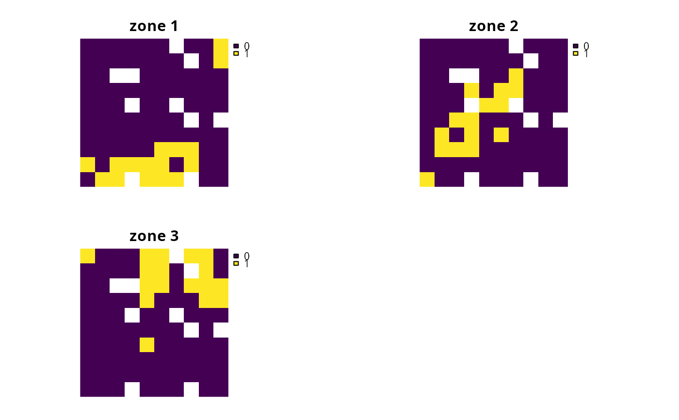
# plot solution
# each panel corresponds to a different zone, and data show the
# status of each planning unit in a given zone
plot(s4, axes = FALSE)


# calculate importance scores
rc4 <- eval_replacement_importance(p4, s4)
names(rc4) <- paste0("zone ", seq_len(terra::nlyr(s4)))

# plot importance
# each panel corresponds to a different zone, and data show the
# importance of each planning unit in a given zone
plot(rc4, axes = FALSE)