Create relative tolerance values for a multi-objective approach
Source:R/approach_rel_tol_matrix.R
approach_rel_tol_matrix.RdCreate multiple sets of relative tolerance values to generate multiple
solutions with the hierarchical approach for multi-objective optimization
(i.e., the rel_tol parameter of add_hier_approach()).
Arguments
- n_problems
integervalue denoting the number ofproblem()objects for which to generate values.- n_values
integerdenoting the number of relative tolerance values to to generate for eachproblem()object (pern_problems), except for the lastproblem().- max
numericpositive value denoting the maximum relative tolerance value. For example, a value of 0.2 means that some of the resulting solutions could perform up to 20% worse than optimality for particular objectives. Similarity, a value of 1.5 means that some of the resulting solutions could perform up to 150% worse than optimality for particular objectives.- include_zeros
logicalvalue indicating if the relative tolerance values should include zeros? Ifinclude_zeros = TRUE, then some of the sets will assign a value of zero to some of the objectives, and so solutions based on these sets will ensure optimality for the objectives with zero values. Defaults toTRUE.- order
logicalvalue indicating if each set returned relative tolerance values should only contain values in descending order of priority. For example, if considering three problems, then a set ofrel_tol = c(0.8, 0.2)would have values in descending order of priority and a set ofrel_tol = c(0.2, 0.8)would not. If you want to generate relative tolerance values to explore trade-offs assuming a particular order of priority when using the hierarchical approach, then we recommend usingorder = TRUE. Defaults toTRUE.
Value
A numeric matrix. Here, rows correspond to
different sets of each relative tolerance values and columns correspond to
different objectives.
Examples
# in this example, we aim to identify a set of planning units that will
# not exceed a particular budget and meet objectives for
# (i) representing species that are important for ecosystem
# functioning (hereafter, keystone species) and (ii) representing species
# that have high social or cultural value (hereafter, iconic species)
# import data
con_cost <- get_sim_pu_raster()
keystone_spp <- get_sim_features()[[1:3]]
iconic_spp <- get_sim_features()[[4:5]]
# define a total conservation budget (30% of total cost)
budget <- terra::global(con_cost, "sum", na.rm = TRUE)[[1]] * 0.3
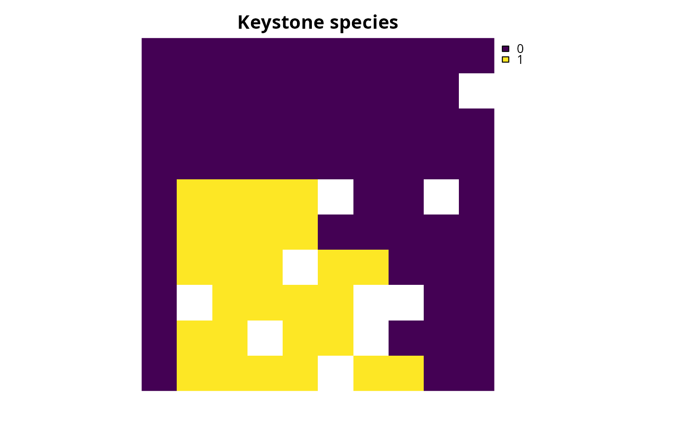
# define a single-objective problem for the keystone species objective
p1 <-
problem(con_cost, keystone_spp) %>%
add_min_shortfall_objective(budget) %>%
add_relative_targets(0.4) %>%
add_binary_decisions()
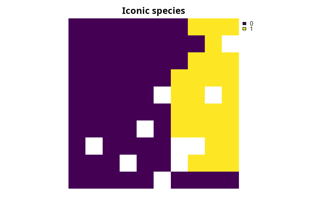
# define a single-objective problem for the iconic species objective
p2 <-
problem(con_cost, iconic_spp) %>%
add_min_shortfall_objective(budget) %>%
add_relative_targets(0.45) %>%
add_binary_decisions()
# solve the single-objective problems
s1 <-
p1 %>%
add_default_solver(verbose = FALSE) %>%
solve()
s2 <-
p2 %>%
add_default_solver(verbose = FALSE) %>%
solve()
# plot the solutions to the single-objective problems
plot(s1, main = "Keystone species", axes = FALSE)
 plot(s2, main = "Iconic species", axes = FALSE)
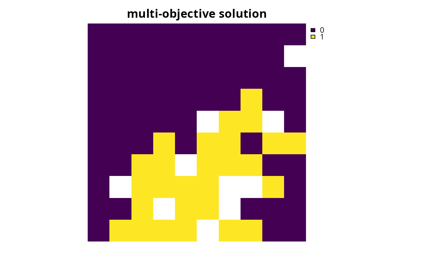
 # now we will a create multi-objective problem that simultaneously
# considers both of these objectives
# the first objective for keystone species will have a higher order of
# priority than the second objective for iconic species -- because
# the long-term persistence of iconic species depends on ecosystem
# functioning -- and we will specify a very small relative tolerance
# parameter so that the solution has a relatively high performance according
# to the first objective (i.e., relatively low representation shortfalls for
# keystone species)
mp1 <-
multi_problem(keystone_obj = p1, iconic_obj = p2) %>%
add_hier_approach(
rel_tol = 0.01,
priority = c(2, 1),
verbose = FALSE
) %>%
add_default_solver(verbose = FALSE)
# solve multi-objective problem
ms1 <- solve(mp1)
# plot solution to multi-objective problem
plot(ms1, main = "multi-objective solution", axes = FALSE)
# now we will a create multi-objective problem that simultaneously
# considers both of these objectives
# the first objective for keystone species will have a higher order of
# priority than the second objective for iconic species -- because
# the long-term persistence of iconic species depends on ecosystem
# functioning -- and we will specify a very small relative tolerance
# parameter so that the solution has a relatively high performance according
# to the first objective (i.e., relatively low representation shortfalls for
# keystone species)
mp1 <-
multi_problem(keystone_obj = p1, iconic_obj = p2) %>%
add_hier_approach(
rel_tol = 0.01,
priority = c(2, 1),
verbose = FALSE
) %>%
add_default_solver(verbose = FALSE)
# solve multi-objective problem
ms1 <- solve(mp1)
# plot solution to multi-objective problem
plot(ms1, main = "multi-objective solution", axes = FALSE)
 # we will explore trade-offs between the two objectives, by generating
# multiple solutions using multi-objective optimization
# create a matrix with multiple different relative tolerance values
rel_tol_matrix <- approach_rel_tol_matrix(
n_problems = 2, n_values = 20, max = 1.2
)
# print matrix with relative tolerance values
print(rel_tol_matrix)
#> [,1]
#> [1,] 0.00000000
#> [2,] 0.06315789
#> [3,] 0.12631579
#> [4,] 0.18947368
#> [5,] 0.25263158
#> [6,] 0.31578947
#> [7,] 0.37894737
#> [8,] 0.44210526
#> [9,] 0.50526316
#> [10,] 0.56842105
#> [11,] 0.63157895
#> [12,] 0.69473684
#> [13,] 0.75789474
#> [14,] 0.82105263
#> [15,] 0.88421053
#> [16,] 0.94736842
#> [17,] 1.01052632
#> [18,] 1.07368421
#> [19,] 1.13684211
#> [20,] 1.20000000
# create a multi-objective problem with the matrix of relative tolerance
# values and - because we do not specify values for priority - the
# optimization process will assume that the objectives are already
# specified in order of priority
mp2 <-
multi_problem(keystone_obj = p1, iconic_obj = p2) %>%
add_hier_approach(rel_tol = rel_tol_matrix, verbose = TRUE) %>%
add_default_solver(gap = 0.01, verbose = FALSE)
# solve multi-objective problem and remove duplicate solutions
ms2 <- solve(mp2, remove_duplicates = TRUE)
#> Generating solutions ■■■■■ | 3/20 | 15% | ETA: 8s
#> Generating solutions ■■■■■■■■■■ | 6/20 | 30% | ETA: 7s
#> Generating solutions ■■■■■■■■■■■■■■■■■■■■■ | 13/20 | 65% | ETA: 3s
#> Generating solutions ■■■■■■■■■■■■■■■■■■■■■■■■■■■■■■■ | 20/20 | 100% | ETA: 0s
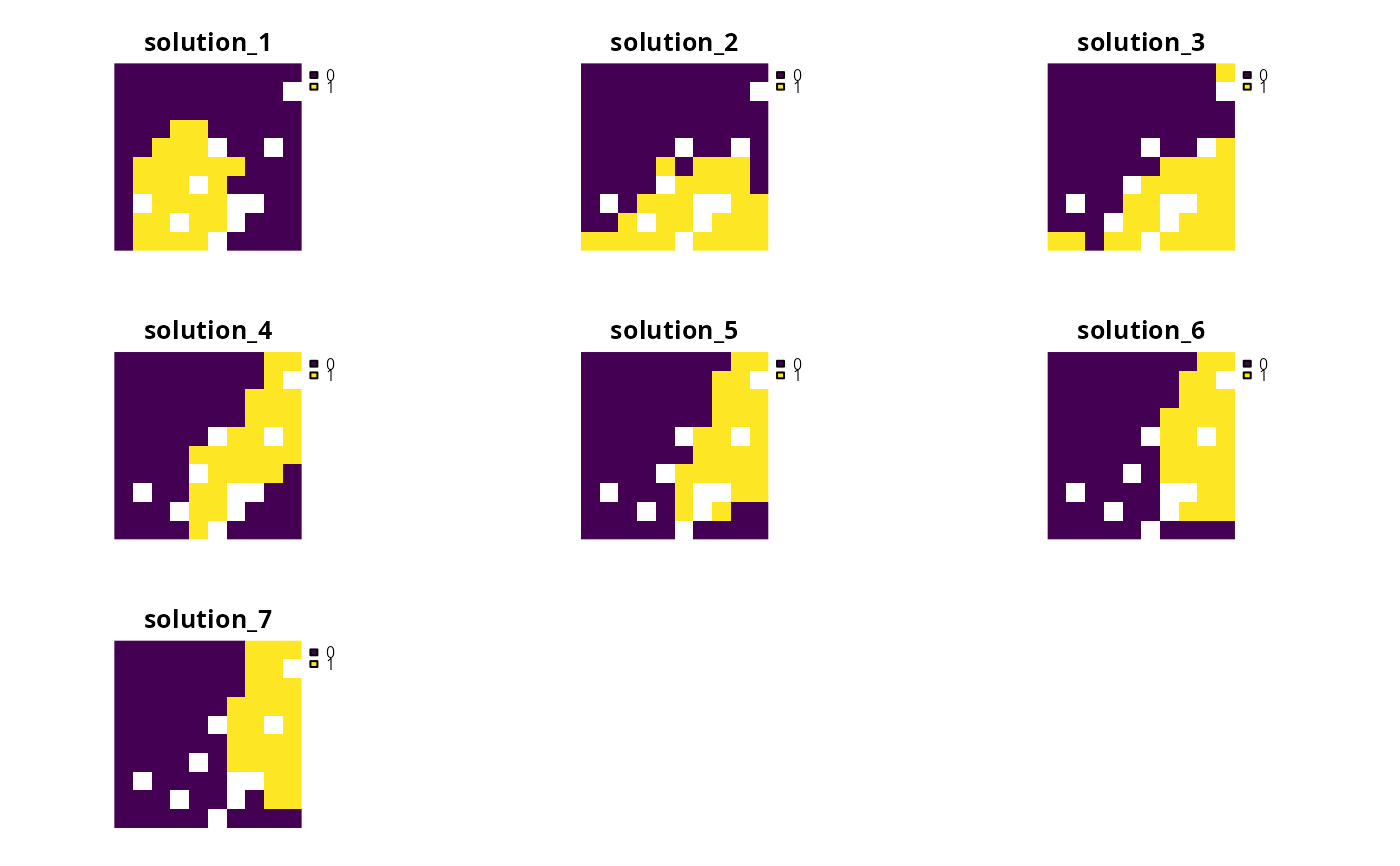
#> ℹ Found 7 out of the requested 20 non-duplicate solutions.
# plot multiple solutions
plot(terra::rast(ms2), axes = FALSE)
# we will explore trade-offs between the two objectives, by generating
# multiple solutions using multi-objective optimization
# create a matrix with multiple different relative tolerance values
rel_tol_matrix <- approach_rel_tol_matrix(
n_problems = 2, n_values = 20, max = 1.2
)
# print matrix with relative tolerance values
print(rel_tol_matrix)
#> [,1]
#> [1,] 0.00000000
#> [2,] 0.06315789
#> [3,] 0.12631579
#> [4,] 0.18947368
#> [5,] 0.25263158
#> [6,] 0.31578947
#> [7,] 0.37894737
#> [8,] 0.44210526
#> [9,] 0.50526316
#> [10,] 0.56842105
#> [11,] 0.63157895
#> [12,] 0.69473684
#> [13,] 0.75789474
#> [14,] 0.82105263
#> [15,] 0.88421053
#> [16,] 0.94736842
#> [17,] 1.01052632
#> [18,] 1.07368421
#> [19,] 1.13684211
#> [20,] 1.20000000
# create a multi-objective problem with the matrix of relative tolerance
# values and - because we do not specify values for priority - the
# optimization process will assume that the objectives are already
# specified in order of priority
mp2 <-
multi_problem(keystone_obj = p1, iconic_obj = p2) %>%
add_hier_approach(rel_tol = rel_tol_matrix, verbose = TRUE) %>%
add_default_solver(gap = 0.01, verbose = FALSE)
# solve multi-objective problem and remove duplicate solutions
ms2 <- solve(mp2, remove_duplicates = TRUE)
#> Generating solutions ■■■■■ | 3/20 | 15% | ETA: 8s
#> Generating solutions ■■■■■■■■■■ | 6/20 | 30% | ETA: 7s
#> Generating solutions ■■■■■■■■■■■■■■■■■■■■■ | 13/20 | 65% | ETA: 3s
#> Generating solutions ■■■■■■■■■■■■■■■■■■■■■■■■■■■■■■■ | 20/20 | 100% | ETA: 0s
#> ℹ Found 7 out of the requested 20 non-duplicate solutions.
# plot multiple solutions
plot(terra::rast(ms2), axes = FALSE)
 # extract objective values for the solutions
obj_matrix <- attributes(ms2)$objective
# print the objective values
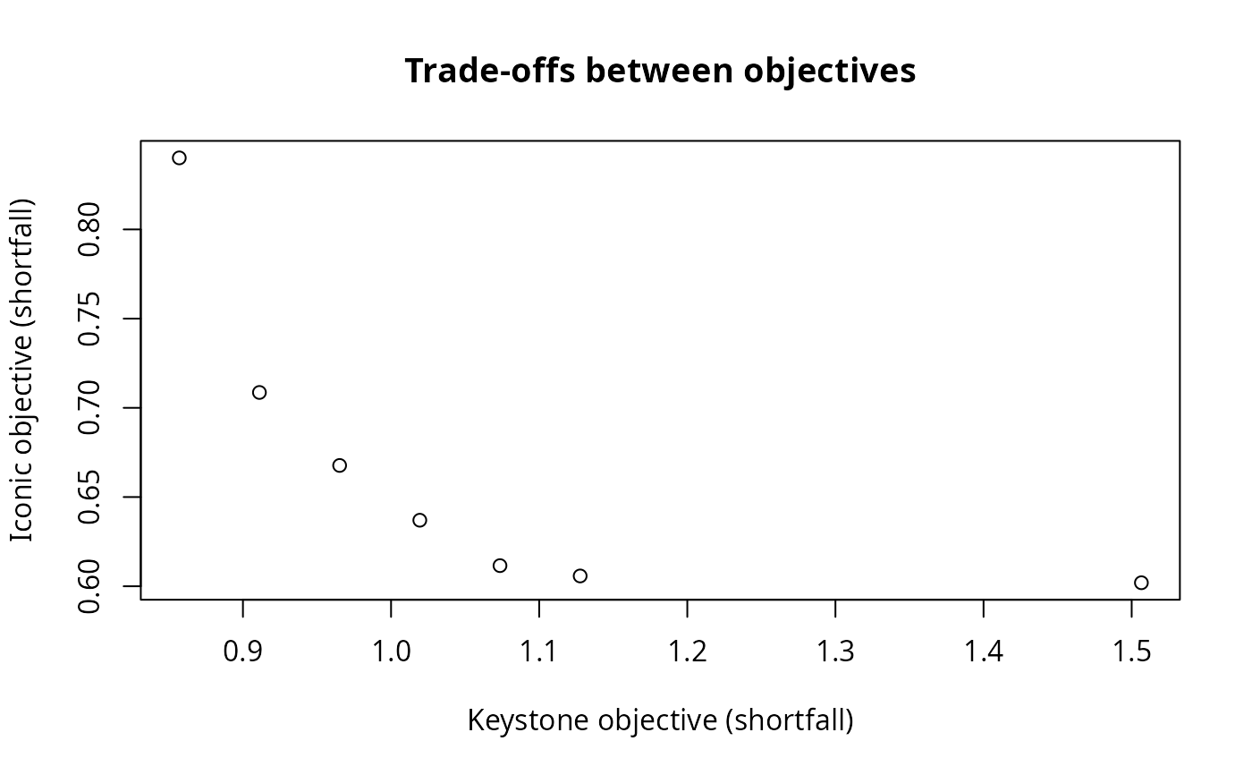
print(obj_matrix)
#> keystone_obj iconic_obj
#> solution_1 0.8570267 0.8400900
#> solution_2 0.9111362 0.7086196
#> solution_3 0.9652827 0.6677060
#> solution_4 1.0194107 0.6370060
#> solution_5 1.0735387 0.6115551
#> solution_6 1.1276667 0.6057715
#> solution_7 1.5065627 0.6019638
# plot the objectives values to visualize trade-offs
# (note that smaller values are better because these objectives seek to
# minimize representation shortfalls)
plot(
obj_matrix,
main = "Trade-offs between objectives",
xlab = "Keystone objective (shortfall)",
ylab = "Iconic objective (shortfall)"
)
# extract objective values for the solutions
obj_matrix <- attributes(ms2)$objective
# print the objective values
print(obj_matrix)
#> keystone_obj iconic_obj
#> solution_1 0.8570267 0.8400900
#> solution_2 0.9111362 0.7086196
#> solution_3 0.9652827 0.6677060
#> solution_4 1.0194107 0.6370060
#> solution_5 1.0735387 0.6115551
#> solution_6 1.1276667 0.6057715
#> solution_7 1.5065627 0.6019638
# plot the objectives values to visualize trade-offs
# (note that smaller values are better because these objectives seek to
# minimize representation shortfalls)
plot(
obj_matrix,
main = "Trade-offs between objectives",
xlab = "Keystone objective (shortfall)",
ylab = "Iconic objective (shortfall)"
)