Specify targets following Wilson et al. (2010)

Specify targets based on the methodology outlined by Wilson et al. (2010). Briefly, this method involves using population growth rate data to set target thresholds based on the amount of habitat required to sustain populations for 100,000 years. To help prevent widespread features from obscuring priorities, targets are capped following Butchart et al. (2015). Note that this function is designed to be used with add_auto_targets() and add_group_targets().

Usage

spec_wilson_targets(
  mean_growth_rates,
  var_growth_rates,
  pop_density,
  density_units,
  cap_area_target = 1e+06,
  area_units = "km^2"
)

Arguments

mean_growth_rates: numeric vector that specifies the average population growth rate that would be expected for each feature within priority areas (i.e., $r$ per Wilson et al. 2010). If a single numeric value is specified, then all features are assigned targets based on the same average population growth rate. See Population growth section for more details.
var_growth_rates: numeric vector that specifies the variance in population growth rate that would be expected for each feature within priority areas (i.e., $\sigma^2$ per Wilson et al. 2010). If a single numeric value is specified, then all features are assigned targets assuming the same variance in population growth rate. See Population growth section for more details.
pop_density: numeric vector that specifies the population density for each feature. If a single numeric value is specified, then all features are assigned targets assuming the same population density. See Population density section for more details.
density_units: character vector that specifies the area-based units for the population density values. For example, units can be used to express that population densities are in terms of individuals per hectare ("ha"), acre ("acre"), or km² ("km^2"). If a single character value is specified, then all features are assigned targets assuming that population density values are in the same units. See Population density section for more details.
cap_area_target: numeric value denoting the area-based target cap. To avoid setting a target cap, a missing (NA) value can be specified. Defaults to 1000000 (i.e., 1,000,000 km²).
area_units: character value denoting the unit of measurement for the area-based arguments. Defaults to "km^2" (i.e., km²).

Value

An object (TargetMethod) for specifying targets that can be used with add_auto_targets() and add_group_targets() to add targets to a problem().

Details

This target setting method was developed to identify the minimum amount of habitat to protect an entire species (Wilson et al. 2010). Although this method was originally applied to the sub-national scale (i.e., the East Kalimantan province of Indonesia), Wilson et al. (2010) linearly re-scaled targets derived from this method according to the proportion of each species' distribution located within the study area (i.e., based on the species' total distribution size in Borneo). As such, this method may especially well-suited for national or global-scale conservation planning exercises, and may also be useful for local-scale planning exercises as long as the targets are re-scaled appropriately. Please note that this function is provided as convenient method to set targets for problems with a single management zone, and cannot be used for those with multiple management zones.

Population growth

This method requires population growth rate data. Although the package does not provide such data, population growth rate estimates can be obtained from published datasets (e.g., Brook et al. 2006). Additionally, population growth rate data may be approximated from physiological traits (e.g., such as body mass, Sinclair 1996; Hilbers et al. 2016). Indeed, Wilson et al. (2010) detail equations for approximating average population growth rate and variance in population growth rate for mammal species based on body mass (based on Sinclair 1996).

Mathematical formulation

This method involves setting target thresholds based on the amount of habitat required to sustain populations for 100,000 years. To express this mathematically, we will define the following terminology. Let $f$ denote the total abundance of a feature (i.e., geographic range size expressed as km²), $k$ the carrying capacity required for a population to persist for 100,000 years, $d$ the population density of the feature (i.e., number of individuals per km², per pop_density and density_units), $r$ the mean population growth rate of the feature inside protected areas (per mean_growth_rates), $\sigma^2$ the variance in population growth rate of the feature inside protected areas (per var_growth_rates), $b$ is a constant calculated from $r$ and $\sigma^2$, and $j$ the target cap (expressed as km², per cap_area_target and area_units). Given this terminology, the target threshold ($t$) for the feature is calculated as follows. $$ t = min(f, min(j, d \times k)) \\ k = (\frac{100000 \times \sigma^2 \times b^2}{2})^\frac{1}{b} \\ b = (2 \times \frac{r}{\sigma^2}) - 1 $$

Data calculations

This function involves calculating targets based on the spatial extent of the features in x. Although it can be readily applied to problem() objects that have the feature data provided as a terra::rast() object, you will need to specify the spatial units for the features when initializing the problem() objects if the feature data are provided in a different format. In particular, if the feature data are provided as a data.frame or character vector, then you will need to specify an argument to feature_units when using the problem() function. See the Examples section of the documentation for add_auto_targets() for a demonstration of specifying the spatial units for features.

Population density

This method requires population density data expressed as the number of individuals per unit area. For example, if a species has 200 individuals per hectare, then this can be specified with pop_density = 200 and density_units = "ha". Alternatively, if a species has a population density where one individual occurs every 10 km², then this can be specified with pop_density = 0.1 and density_units = "km^2". Also, note that population density is assumed to scale linearly with the values in the feature data. For example, if a planning unit contains 5 km² of habitat for a feature, pop_density = 200, and density_units = "km^2", then the calculations assume that the planning unit contains 100 individuals for the species. Although the package does not provide the population density data required to apply this target setting method, such data can be obtained from published databases (e.g., Santini et al. 2022, 2023, 2024; Witting et al. 2024).

References

Brook BW, Traill LW, Bradshaw CJA (2006) Minimum viable population sizes and global extinction risk are unrelated. Ecology Letters, 9:375–382.

Butchart SHM, Clarke M, Smith RJ, Sykes RE, Scharlemann JPW, Harfoot M, Buchanan GM, Angulo A, Balmford A, Bertzky B, Brooks TM, Carpenter KE, Comeros‐Raynal MT, Cornell J, Ficetola GF, Fishpool LDC, Fuller RA, Geldmann J, Harwell H, Hilton‐Taylor C, Hoffmann M, Joolia A, Joppa L, Kingston N, May I, Milam A, Polidoro B, Ralph G, Richman N, Rondinini C, Segan DB, Skolnik B, Spalding MD, Stuart SN, Symes A, Taylor J, Visconti P, Watson JEM, Wood L, Burgess ND (2015) Shortfalls and solutions for meeting national and global conservation area targets. Conservation Letters, 8: 329–337.

Hilbers JP, Santini L, Visconti P, Schipper AM, Pinto C, Rondinini C, Huijbregts MAJ (2016) Setting population targets for mammals using body mass as a predictor of population persistence. Conservation Biology, 31:385–393.

IUCN (2025) The IUCN Red List of Threatened Species. Version 2025-1. Available at https://www.iucnredlist.org. Accessed on 23 July 2025.

Santini L, Mendez Angarita VY, Karoulis C, Fundarò D, Pranzini N, Vivaldi C, Zhang T, Zampetti A, Gargano SJ, Mirante D, Paltrinieri L (2024) TetraDENSITY 2.0—A database of population density estimates in tetrapods. Global Ecology and Biogeography, 33:e13929.

Santini L, Benítez‐López A, Dormann CF, Huijbregts MAJ (2022) Population density estimates for terrestrial mammal species. Global Ecology and Biogeography, 31:978–994.

Santini L, Tobias JA, Callaghan C, Gallego‐Zamorano J, Benítez‐López A (2023) Global patterns and predictors of avian population density. Global Ecology and Biogeography, 32:1189—1204.

Sinclair ARE (1996) Mammal populations: fluctuation, regulation, life history theory and their implications for conservation. In Frontiers of Population Ecology. Floyd RB,Sheppard AW, de Barro PJ (Eds.). Melbourne, Australia: CSIRO Publishing.

Wilson KA, Meijaard E, Drummond S, Grantham HS, Boitani L, Catullo G, Christie L, Dennis R, Dutton I, Falcucci A, Maiorano L, Possingham HP, Rondinini C, Turner WR, Venter O, Watts M (2010) Conserving biodiversity in production landscapes. Ecological Applications, 20:1721–1732.

Witting L (2024) Population dynamic life history models of the birds and mammals of the world. Ecological Informatics, 80:102492.

Examples

# \dontrun{
# set seed for reproducibility
set.seed(500)

# load data
sim_complex_pu_raster <- get_sim_complex_pu_raster()
sim_complex_features <- get_sim_complex_features()

# simulate mean population growth rate data for each feature
sim_mean_growth_rates <- runif(terra::nlyr(sim_complex_features), 1, 3.0)

# simulate variance in population growth rate data for each feature
sim_var_growth_rates <- runif(terra::nlyr(sim_complex_features), 1.0, 2.0)

# simulate population density data for each feature,
# expressed as number of individuals per km^2
sim_pop_density_per_km2 <- runif(terra::nlyr(sim_complex_features), 10, 100)

# create problem with targets based on Wilson et al. (2010)
p1 <-
  problem(sim_complex_pu_raster, sim_complex_features) %>%
  add_min_set_objective() %>%
  add_auto_targets(
    method = spec_wilson_targets(
      mean_growth_rate = sim_mean_growth_rates,
      var_growth_rates = sim_var_growth_rates,
      pop_density = sim_pop_density_per_km2,
      density_units = "km^2"
    )
  ) %>%
  add_binary_decisions() %>%
  add_default_solver(verbose = FALSE)

# solve problem
s1 <- solve(p1)

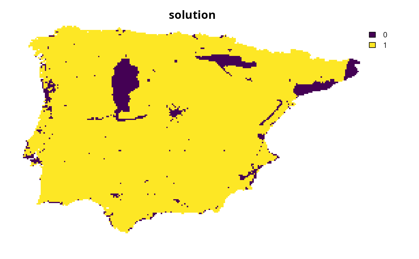
# plot solution
plot(s1, main = "solution", axes = FALSE)

# }