Add targets to a conservation planning problem, wherein each
feature is assigned to a particular group and a target setting
method is specified for each feature group.
This function is designed to provide a convenient alternative to
add_auto_targets().
Arguments
- x
problem()object.- groups
charactervector of group names.- method
listof name-value pairs that describe the target setting method for each group. Here, the names ofmethodcorrespond to different values ingroups. Additionally, the elements ofmethodshould be thecharacternames of target setting methods, or objects (TargetMethod) that specify target setting methods. See Target methods below for more information.
Value
An updated problem() object with the targets added to it.
Target methods
Here method is used to specify a target setting method for each group.
In particular, each element should correspond to a different group,
with the name of the element indicating the group and the value
denoting the target setting method. One option for specifying a
particular target setting method is to use a character value
that denotes the name of the method (e.g., "jung" to set targets following
Jung et al. 2021). This option is particularly useful if default
parameters should be considered during target calculations.
Alternatively, another option for specifying a particular target setting
method is to use a function to define an object (e.g.,
spec_jung_targets() to set targets following Jung et al. 2021).
This alternative option is particularly useful
if customized parameters should be considered during target calculations.
Note that a method can contain a mix of target setting methods defined
using character values and functions.
The following character values can be used to specify target setting
methods:
"jung" (per Jung et al. 2021), "polak"
(per Polak et al. 2016), "rodrigues" (per Rodrigues et al. 2004),
"sreekar" (per Sreekar and Watson 2026),
"ward" (per Ward et al. 2025), and "watson"
(per Watson et al. 2010).
(2010). Additionally, the following values can be used to set targets
based on criteria from the
IUCN Red List of Threatened Species (IUCN 2025):
"rl_species_VU_A1_B1" "rl_species_EN_A1_B1", "rl_species_CR_A1_B1",
"rl_species_VU_A1_B2" "rl_species_EN_A1_B2", "rl_species_CR_A1_B2",
"rl_species_VU_A2_B1" "rl_species_EN_A2_B1", "rl_species_CR_A2_B1",
"rl_species_VU_A2_B2" "rl_species_EN_A2_B2", "rl_species_CR_A2_B2",
"rl_species_VU_A3_B1" "rl_species_EN_A3_B1", "rl_species_CR_A3_B1",
"rl_species_VU_A3_B2" "rl_species_EN_A3_B2", "rl_species_CR_A3_B2",
"rl_species_VU_A4_B1" "rl_species_EN_A4_B1", "rl_species_CR_A4_B1",
"rl_species_VU_A4_B2" "rl_species_EN_A4_B2", and
"rl_species_CR_A4_B2".
Furthermore, the following values can be used to set targets based on
criteria from the IUCN Red List of Ecosystems (IUCN 2024):
"rl_ecosystem_VU_A1_B1", "rl_ecosystem_EN_A1_B1",
"rl_ecosystem_CR_A1_B1",
"rl_ecosystem_VU_A1_B2", "rl_ecosystem_EN_A1_B2",
"rl_ecosystem_CR_A1_B2",
"rl_ecosystem_VU_a2a_B1", "rl_ecosystem_EN_a2a_B1",
"rl_ecosystem_CR_a2a_B1",
"rl_ecosystem_VU_a2a_B2", "rl_ecosystem_EN_a2a_B2",
"rl_ecosystem_CR_a2a_B2",
"rl_ecosystem_VU_a2b_B1", "rl_ecosystem_EN_a2b_B1",
"rl_ecosystem_CR_a2b_B1",
"rl_ecosystem_VU_a2b_B2", "rl_ecosystem_EN_a2b_B2",
"rl_ecosystem_CR_a2b_B2",
"rl_ecosystem_VU_A3_B1", "rl_ecosystem_EN_A3_B1",
"rl_ecosystem_CR_A3_B1",
"rl_ecosystem_VU_A3_B2", "rl_ecosystem_EN_A3_B2", and
"rl_ecosystem_CR_A3_B2".'
For convenience, these options can also be specified with lower case letters (e.g., "rl_species_VU_A1_B1" may alternatively be specified as "rl_species_vu_a1_b1").
Note that target setting methods that require additional data or parameters cannot be specified with character values.
The following functions can be used to create an object for specifying
a target setting method: spec_absolute_targets(), spec_relative_targets(),
spec_area_targets(), spec_interp_absolute_targets(),
spec_interp_area_targets(),
spec_duran_targets(), spec_jung_targets(), spec_polak_targets(),
spec_pop_size_targets(),
spec_rl_ecosystem_targets(), spec_rl_species_targets(),
spec_rodrigues_targets(),
spec_rule_targets(), spec_sreekar_targets(), spec_ward_targets(),
spec_watson_targets(), spec_wilson_targets(), spec_min_targets(), and
spec_max_targets().
Target setting
Many conservation planning problems require targets. Targets are used to specify the minimum amount, or proportion, of a feature's spatial distribution that should ideally be protected. This is important so that the optimization process can weigh the merits and trade-offs between improving the representation of one feature over another feature. Although it can be challenging to set meaningful targets, this is a critical step for ensuring that prioritizations meet the stakeholder objectives that underpin a prioritization exercise (Carwardine et al. 2009). In other words, targets play an important role in ensuring that a priority setting process is properly tuned according to stakeholder requirements. For example, targets provide a mechanism for ensuring that a prioritization secures enough habitat to promote the long-term persistence of each threatened species, culturally important species, or economically important ecosystem services under consideration. Since there is often uncertainty regarding stakeholder objectives (e.g., how much habitat should be protected for a given species) or the influence of particular target on a prioritization (e.g., how would setting a 90% or 100% for a threatened species alter priorities), it is often useful to generate and compare a suite of prioritizations based on different target scenarios.
Data calculations
Many of the functions for specifying target setting methods involve
calculating targets based on the spatial extent of the features in x
(e.g., spec_jung_targets(), [spec_rodrigues_targets(), and others).
Although this function for adding targets can be readily applied to
problem() objects that
have the feature data provided as a terra::rast() object,
you will need to specify the spatial units for the features
when building a problem() object if the feature data
are provided in a different format. In particular, if the feature
data are provided as a data.frame or character vector,
then you will need to specify feature_units when
using the problem() function. See the Examples section below for a
demonstration of using the feature_units parameter.
References
Carwardine J, Klein CJ, Wilson KA, Pressey RL, Possingham HP (2009) Hitting the target and missing the point: target‐based conservation planning in context. Conservation Letters, 2: 4–11.
Jung M, Arnell A, de Lamo X, García-Rangel S, Lewis M, Mark J, Merow C, Miles L, Ondo I, Pironon S, Ravilious C, Rivers M, Schepaschenko D, Tallowin O, van Soesbergen A, Govaerts R, Boyle BL, Enquist BJ, Feng X, Gallagher R, Maitner B, Meiri S, Mulligan M, Ofer G, Roll U, Hanson JO, Jetz W, Di Marco M, McGowan J, Rinnan DS, Sachs JD, Lesiv M, Adams VM, Andrew SC, Burger JR, Hannah L, Marquet PA, McCarthy JK, Morueta-Holme N, Newman EA, Park DS, Roehrdanz PR, Svenning J-C, Violle C, Wieringa JJ, Wynne G, Fritz S, Strassburg BBN, Obersteiner M, Kapos V, Burgess N, Schmidt- Traub G, Visconti P (2021) Areas of global importance for conserving terrestrial biodiversity, carbon and water. Nature Ecology and Evolution, 5:1499–1509.
Polak T, Watson JEM, Fuller RA, Joseph LN, Martin TG, Possingham HP, Venter O, Carwardine J (2015) Efficient expansion of global protected areas requires simultaneous planning for species and ecosystems. Royal Society Open Science, 2: 150107.
See also
Other functions for adding targets:
add_absolute_targets(),
add_auto_targets(),
add_manual_targets(),
add_relative_targets()
Examples
# set seed for reproducibility
set.seed(500)
# load data
sim_complex_pu_raster <- get_sim_complex_pu_raster()
sim_complex_features <- get_sim_complex_features()
sim_pu_polygons <- get_sim_pu_polygons()
# create grouping data, wherein each feature will be randomly
# assigned to the group A, B, C, or D
sim_groups <- sample(
c("A", "B", "C", "D"), terra::nlyr(sim_complex_features), replace = TRUE
)
# create problem where each feature in group A is assigned a 20% target,
# each feature in group B is assigned a target based on Jung et al. (2021),
# each feature in group C is assigned a target based on Ward et al. (2025),
# and each feature in group D is assigned a target based on Rodrigues
# et al. (2004)
p1 <-
problem(sim_complex_pu_raster, sim_complex_features) %>%
add_min_set_objective() %>%
add_group_targets(
groups = sim_groups,
method = list(
A = spec_relative_targets(0.2),
B = spec_jung_targets(),
C = spec_ward_targets(),
D = spec_rodrigues_targets()
)
) %>%
add_binary_decisions() %>%
add_default_solver(verbose = FALSE)
# solve problem
s1 <- solve(p1)
# plot solution
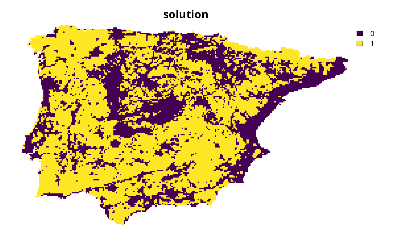
plot(s1, main = "solution", axes = FALSE)
 # here we will show how to set the feature_units when the feature
# are not terra::rast() objects. in this example, we have planning units
# stored in an sf object (i.e., sim_pu_polygons) and the feature data will
# be stored as columns in the sf object.
# we will start by simulating feature data for the planning units.
# in particular, the simulated values will describe the amount of habitat
# for each feature expressed as acres (e.g., a value of 30 means 30 acres).
sim_pu_polygons$feature_1 <- runif(nrow(sim_pu_polygons), 0, 500)
sim_pu_polygons$feature_2 <- runif(nrow(sim_pu_polygons), 0, 600)
sim_pu_polygons$feature_3 <- runif(nrow(sim_pu_polygons), 0, 300)
# we will now build a problem with these data and specify the
# the feature units as acres because that those are the units we
# used for simulating the data. also, we will specify targets
# of 2 km^2 of habitat for the first feature, and 3 km^2 for the
# remaining two features by assigning the features to groups.
# although the feature units are acres, the function is able to able
# to automatically convert the units.
p2 <-
problem(
sim_pu_polygons,
c("feature_1", "feature_2", "feature_3"),
cost_column = "cost",
feature_units = "acres"
) %>%
add_min_set_objective() %>%
add_group_targets(
groups = c("A", "B", "B"),
method = list(
A = spec_area_targets(targets = 2, area_units = "km^2"),
B = spec_area_targets(targets = 3, area_units = "km^2")
)
) %>%
add_binary_decisions() %>%
add_default_solver(gap = 0, verbose = FALSE)
# solve problem
s2 <- solve(p2)
# plot solution
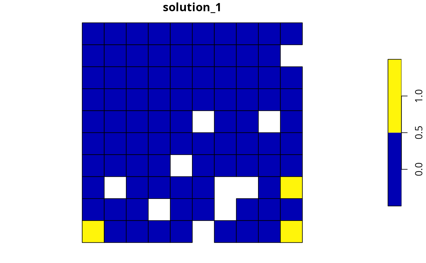
plot(s2[, "solution_1"], axes = FALSE)
# here we will show how to set the feature_units when the feature
# are not terra::rast() objects. in this example, we have planning units
# stored in an sf object (i.e., sim_pu_polygons) and the feature data will
# be stored as columns in the sf object.
# we will start by simulating feature data for the planning units.
# in particular, the simulated values will describe the amount of habitat
# for each feature expressed as acres (e.g., a value of 30 means 30 acres).
sim_pu_polygons$feature_1 <- runif(nrow(sim_pu_polygons), 0, 500)
sim_pu_polygons$feature_2 <- runif(nrow(sim_pu_polygons), 0, 600)
sim_pu_polygons$feature_3 <- runif(nrow(sim_pu_polygons), 0, 300)
# we will now build a problem with these data and specify the
# the feature units as acres because that those are the units we
# used for simulating the data. also, we will specify targets
# of 2 km^2 of habitat for the first feature, and 3 km^2 for the
# remaining two features by assigning the features to groups.
# although the feature units are acres, the function is able to able
# to automatically convert the units.
p2 <-
problem(
sim_pu_polygons,
c("feature_1", "feature_2", "feature_3"),
cost_column = "cost",
feature_units = "acres"
) %>%
add_min_set_objective() %>%
add_group_targets(
groups = c("A", "B", "B"),
method = list(
A = spec_area_targets(targets = 2, area_units = "km^2"),
B = spec_area_targets(targets = 3, area_units = "km^2")
)
) %>%
add_binary_decisions() %>%
add_default_solver(gap = 0, verbose = FALSE)
# solve problem
s2 <- solve(p2)
# plot solution
plot(s2[, "solution_1"], axes = FALSE)