Systematic Conservation Prioritization in R
The prioritizr R package uses mixed integer linear programming (MILP) techniques to provide a flexible interface for building and solving conservation planning problems. It supports a broad range of objectives, constraints, and penalties that can be used to custom-tailor conservation planning problems to the specific needs of a conservation planning exercise. Once built, conservation planning problems can be solved using a variety of commercial and open-source exact algorithm solvers. In contrast to the algorithms conventionally used to solve conservation problems, such as heuristics or simulated annealing, the exact algorithms used here are guaranteed to find optimal solutions. Furthermore, conservation problems can be constructed to optimize the spatial allocation of different management actions or zones, meaning that conservation practitioners can identify solutions that benefit multiple stakeholders. Finally, this package has the functionality to read input data formatted for the Marxan conservation planning program, and find much cheaper solutions in a much shorter period of time than Marxan.
Installation
Official version
The latest official version of the prioritizr R package can be installed from the Comprehensive R Archive Network (CRAN) using the following R code.
install.packages("prioritizr", repos = "https://cran.rstudio.com/")Developmental version
The latest development version can be installed to gain access to new functionality that is not yet present in the latest official version. Please note that the developmental version is more likely to contain coding errors than the official version. To install the developmental version, you can install it directly from the GitHub online code repository or from the R Universe. In general, we recommend installing the developmental version from the R Universe. This is because installation via R Universe does not require any additional software (e.g., RTools for Windows systems, or Xcode and gfortran for macOS systems).
-
To install the latest development version from R Universe, use the following R code.
install.packages( "prioritizr", repos = c( "https://prioritizr.r-universe.dev", "https://cloud.r-project.org" ) ) -
To install the latest development version from GitHub, use the following R code.
if (!require(remotes)) install.packages("remotes")
remotes::install_github("prioritizr/prioritizr")
Citation
Please cite the prioritizr R package when using it in publications. To cite the package, please use:
Hanson JO, Schuster R, Strimas‐Mackey M, Morrell N, Edwards BPM, Arcese P, Bennett JR, and Possingham HP (2025) Systematic conservation prioritization with the prioritizr R package. Conservation Biology, 39: e14376.
Additionally, we keep a record of publications that use the prioritizr R package. If you use this package in any reports or publications, please file an issue on GitHub so we can add it to the record.
Usage
Here we provide a short example showing how the prioritizr R package can be used to build and solve conservation problems. Specifically, we will use an example dataset available through the prioritizrdata R package. Additionally, we will use the terra R package to perform raster calculations. To begin with, we will load the packages.
# load packages
library(prioritizr)
library(prioritizrdata)
library(terra)
We will use the Washington dataset in this example. To import the planning unit data, we will use the get_wa_pu() function. Although the prioritizr R package can support many different types of planning unit data, here our planning units are represented as a single-layer raster (i.e., terra::rast() object). Each cell represents a different planning unit, and cell values denote land acquisition costs. Specifically, there are 10757 planning units in total (i.e., cells with non-missing values).
## class       : SpatRaster
## size        : 109, 147, 1  (nrow, ncol, nlyr)
## resolution  : 4000, 4000  (x, y)
## extent      : -1816382, -1228382, 247483.5, 683483.5  (xmin, xmax, ymin, ymax)
## coord. ref. : +proj=laea +lat_0=45 +lon_0=-100 +x_0=0 +y_0=0 +ellps=sphere +units=m +no_defs
## source      : wa_pu.tif
## name        :         cost
## min value   :    0.2986647
## max value   : 1804.1838379
# plot data
plot(wa_pu, main = "Costs", axes = FALSE)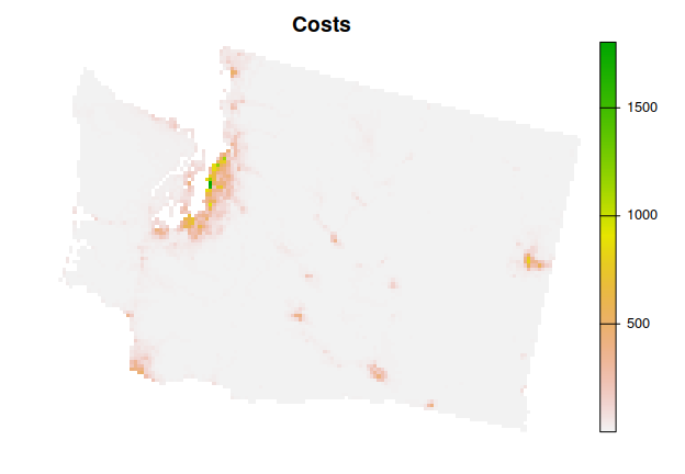
Next, we will use the get_wa_features() function to import the conservation feature data. Although the prioritizr R package can support many different types of feature data, here our feature data are represented as a multi-layer raster (i.e., terra::rast() object). Each layer describes the spatial distribution of a feature. Here, our feature data correspond to different bird species. To account for migratory patterns, the breeding and non-breeding distributions of species are represented as different features. Specifically, the cell values denote the relative abundance of individuals, with higher values indicating greater abundance.
# import feature data
wa_features <- get_wa_features()

# preview data
print(wa_features)
## class : SpatRaster
## size : 109, 147, 396 (nrow, ncol, nlyr)
## resolution : 4000, 4000 (x, y)
## extent : -1816382, -1228382, 247483.5, 683483.5 (xmin, xmax, ymin, ymax)
## coord. ref. : +proj=laea +lat_0=45 +lon_0=-100 +x_0=0 +y_0=0 +ellps=sphere +units=m +no_defs
## source : wa_features.tif
## names : Recur~ding), Botau~ding), Botau~ding), Corvu~ding), Corvu~ding), Cincl~full), ...
## min values : 0.000, 0.000, 0.000, 0.000, 0.000, 0.00, ...
## max values : 0.514, 0.812, 3.129, 0.115, 0.296, 0.06, ...
# plot the first nine features
plot(wa_features[[1:9]], nr = 3, axes = FALSE)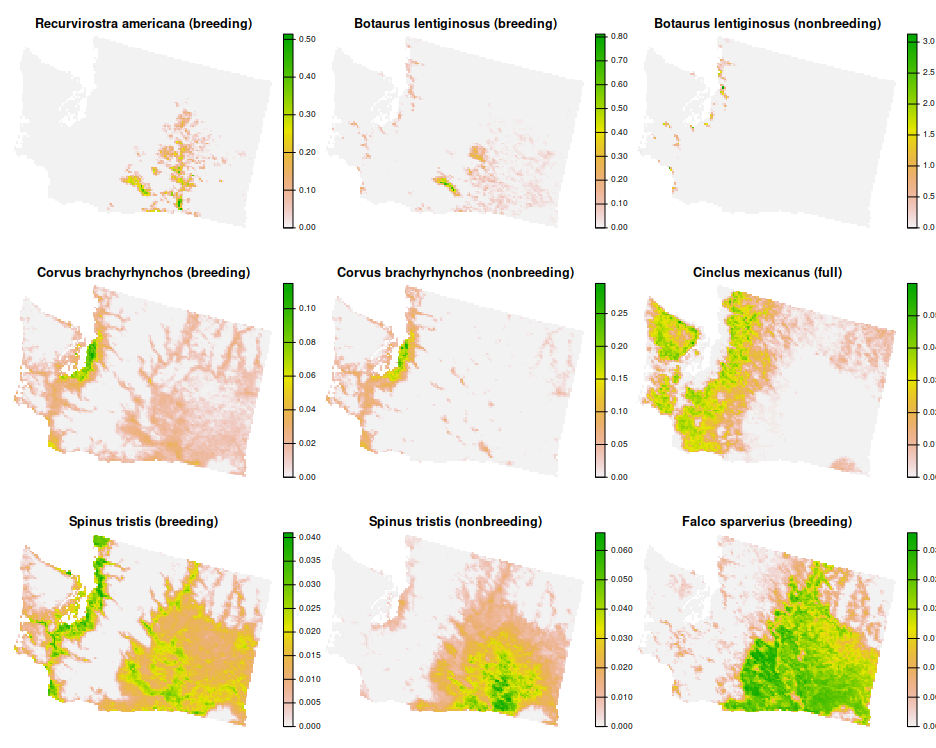
Let’s make sure that you have a solver installed on your computer. This is important so that you can use optimization algorithms to generate spatial prioritizations. If this is your first time using the prioritizr R package, please install the HiGHS solver using the following R code. Although the HiGHS solver is relatively fast and easy to install, please note that you’ll need to install the Gurobi software suite and the gurobi R package for best performance (see the Gurobi Installation Guide for details).
# if needed, install HiGHS solver
install.packages("highs", repos = "https://cran.rstudio.com/")
Now, let’s generate a spatial prioritization. To ensure feasibility, we will set a budget. Specifically, the total cost of the prioritization will represent a 5% of the total land value in the study area. Given this budget, we want the prioritization to increase feature representation, as much as possible, so that each feature would, ideally, have 20% of its distribution covered by the prioritization. In this scenario, we can either purchase all of the land inside a given planning unit, or none of the land inside a given planning unit. Thus we will create a new problem() that will use a minimum shortfall objective (via add_min_shortfall_objective()), with relative targets of 20% (via add_relative_targets()), binary decisions (via add_binary_decisions()), and specify that we want near-optimal solutions (i.e., 10% from optimality) using the best solver installed on our computer (via add_default_solver()).
# calculate budget
budget <- terra::global(wa_pu, "sum", na.rm = TRUE)[[1]] * 0.05

# create problem
p1 <-
  problem(wa_pu, features = wa_features) %>%
  add_min_shortfall_objective(budget) %>%
  add_relative_targets(0.2) %>%
  add_binary_decisions() %>%
  add_default_solver(gap = 0.1, verbose = FALSE)

# print problem
print(p1)
## A conservation problem (<ConservationProblem>)
## ├•data
## │├•features: "Recurvirostra americana (breeding)", … (396 total)
## │└•planning units:
## │ ├•data: <SpatRaster> (10757 total)
## │ ├•costs: continuous values (between 0.2986647 and 1804.184)
## │ ├•extent: -1816382, 247483.5, -1228382, 683483.5 (xmin, ymin, xmax, ymax)
## │ └•CRS: +proj=laea +lat_0=45 +lon_0=-100 +x_0=0 +y_0=0 +ellps=sphere +units=m +no_defs (projected)
## ├•formulation
## │├•objective: minimum shortfall objective (`budget` = 8748.491)
## │├•penalties: none specified
## │├•features:
## ││├•targets: relative targets (all equal to 0.2)
## ││└•weights: none specified
## │├•constraints: none specified
## │└•decisions: binary decision
## └•optimization
## ├•portfolio: default portfolio
## └•solver: gurobi solver (`gap` = 0.1, `time_limit` = 2147483647, `first_feasible` = FALSE, …)
## # ℹ Use `summary(...)` to see complete formulation.After we have built a problem(), we can solve it to obtain a solution.
# plot the solution
plot(s1, main = "Solution", axes = FALSE)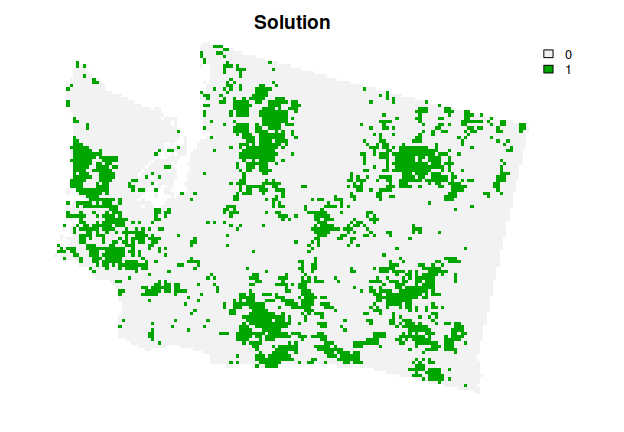
After generating a solution, it is important to evaluate it. Here, we will calculate the number of planning units selected by the solution, and the total cost of the solution. We can also check how many representation targets are met by the solution.
# calculate number of selected planning units by solution
eval_n_summary(p1, s1)
# calculate total cost of solution
eval_cost_summary(p1, s1)
# calculate target coverage for the solution
p1_target_coverage <- eval_target_coverage_summary(p1, s1)
print(p1_target_coverage)
## # A tibble: 396 × 9
## feature met total_amount absolute_target absolute_held absolute_shortfall
## <chr> <lgl> <dbl> <dbl> <dbl> <dbl>
## 1 Recurvir… TRUE 100. 20.0 23.4 0
## 2 Botaurus… TRUE 99.9 20.0 29.2 0
## 3 Botaurus… TRUE 100. 20.0 34.0 0
## 4 Corvus b… TRUE 99.9 20.0 20.4 0
## 5 Corvus b… FALSE 99.9 20.0 18.5 1.46
## 6 Cinclus … TRUE 100. 20.0 20.5 0
## 7 Spinus t… TRUE 99.9 20.0 22.6 0
## 8 Spinus t… TRUE 99.9 20.0 23.1 0
## 9 Falco sp… TRUE 99.9 20.0 24.9 0
## 10 Falco sp… TRUE 100.0 20.0 24.5 0
## # ℹ 386 more rows
## # ℹ 3 more variables: relative_target <dbl>, relative_held <dbl>,
## # relative_shortfall <dbl>
# check percentage of the features that have their target met given the solution
print(mean(p1_target_coverage$met) * 100)Although this solution helps meet the representation targets, it does not account for existing protected areas inside the study area. As such, it does not account for the possibility that some features could be partially – or even fully – represented by existing protected areas and, in turn, might fail to identify meaningful priorities for new protected areas. To address this issue, we will use the get_wa_locked_in() function to import spatial data for protected areas in the study area. We will then add constraints to the problem() to ensure they are selected by the solution (via add_locked_in_constraints()).
# import locked in data
wa_locked_in <- get_wa_locked_in()

# print data
print(wa_locked_in)
## class : SpatRaster
## size : 109, 147, 1 (nrow, ncol, nlyr)
## resolution : 4000, 4000 (x, y)
## extent : -1816382, -1228382, 247483.5, 683483.5 (xmin, xmax, ymin, ymax)
## coord. ref. : +proj=laea +lat_0=45 +lon_0=-100 +x_0=0 +y_0=0 +ellps=sphere +units=m +no_defs
## source : wa_locked_in.tif
## name : protected areas
## min value : 0
## max value : 1
# plot data
plot(wa_locked_in, main = "Existing protected areas", axes = FALSE)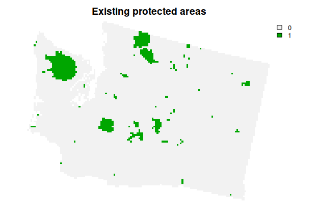
# create new problem with locked in constraints added to it
p2 <-
  p1 %>%
  add_locked_in_constraints(wa_locked_in)

# solve the problem
s2 <- solve(p2)

# plot the solution
plot(s2, main = "Solution", axes = FALSE)
This solution is an improvement over the previous solution. However, there are some places in the study area that are not available for protected area establishment (e.g., due to land tenure). As a consequence, the solution might not be practical for implementation, because it might select some places that are not available for protection. To address this issue, we will use the get_wa_locked_out() function to import spatial data describing which planning units are not available for protection. We will then add constraints to the problem() to ensure they are not selected by the solution (via add_locked_out_constraints()).
# import locked out data
wa_locked_out <- get_wa_locked_out()

# print data
print(wa_locked_out)
## class : SpatRaster
## size : 109, 147, 1 (nrow, ncol, nlyr)
## resolution : 4000, 4000 (x, y)
## extent : -1816382, -1228382, 247483.5, 683483.5 (xmin, xmax, ymin, ymax)
## coord. ref. : +proj=laea +lat_0=45 +lon_0=-100 +x_0=0 +y_0=0 +ellps=sphere +units=m +no_defs
## source : wa_locked_out.tif
## name : urban areas
## min value : 0
## max value : 1
# plot data
plot(wa_locked_out, main = "Areas not available for protection", axes = FALSE)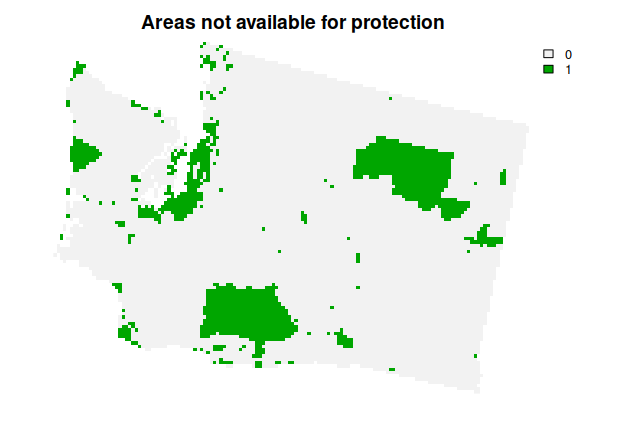
# create new problem with locked out constraints added to it
p3 <-
  p2 %>%
  add_locked_out_constraints(wa_locked_out)

# solve the problem
s3 <- solve(p3)

# plot the solution
plot(s3, main = "Solution", axes = FALSE)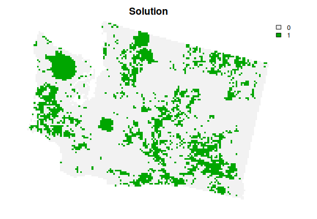
This solution is even better then the previous solution. However, we are not finished yet. The planning units selected by the solution are fairly fragmented. This can cause issues because fragmentation increases management costs and reduces conservation benefits through edge effects. To address this issue, we can further modify the problem by adding penalties that punish overly fragmented solutions (via add_boundary_penalties()). Here we will use a penalty factor (i.e., boundary length modifier) of 0.003, and an edge factor of 50% so that planning units that occur on the outer edge of the study area are not overly penalized.
# create new problem with boundary penalties added to it
p4 <-
  p3 %>%
  add_boundary_penalties(penalty = 0.003, edge_factor = 0.5)

# solve the problem
s4 <- solve(p4)

# plot the solution
plot(s4, main = "Solution", axes = FALSE)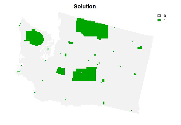
Now, let’s explore which planning units selected by the solution are most important for cost-effectively meeting the targets. To achieve this, we will calculate importance (irreplaceability) scores using an incremental rank approach. Briefly, the optimization problem is solved multiple times in an incremental process with increasing budgets, and planning units are assigned ranks based on which increment they are selected in. Planning units selected earlier on in the process are considered more important.
# calculate importance scores
imp <-
  p4 %>%
  eval_rank_importance(s4, n = 5)

# print scores
print(imp)
## class : SpatRaster
## size : 109, 147, 1 (nrow, ncol, nlyr)
## resolution : 4000, 4000 (x, y)
## extent : -1816382, -1228382, 247483.5, 683483.5 (xmin, xmax, ymin, ymax)
## coord. ref. : +proj=laea +lat_0=45 +lon_0=-100 +x_0=0 +y_0=0 +ellps=sphere +units=m +no_defs
## source(s) : memory
## varname : wa_pu
## name : rs
## min value : 0
## max value : 1
# set planning units that are locked in to -1 so we can easily
# see importance scores for priority areas
imp <- terra::mask(imp, s4, maskvalues = 0, updatevalue = -1)

# plot the total importance scores
## planning units shown in purple were not selected in solution s4
## planning units shown in blue are less important
## planning units shown in yellow are highly important
## note that locked in planning units are also shown in yellow
plot(imp, axes = FALSE,  main = "Importance scores")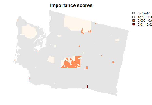
This short example demonstrates how the prioritizr R package can be used to build and customize conservation problems, and then solve them to generate solutions. Although we explored just a few different functions for modifying a conservation problem, the package provides many functions for specifying objectives, constraints, penalties, and decision variables, so that you can build and custom-tailor conservation planning problems to suit your planning scenario.
Learning resources
The package website contains information on the prioritizr R package. Here you can find documentation for every function and built-in dataset, and news describing the updates in each package version. It also contains the following articles and tutorials.
- Getting started: Short tutorial on using the package.
- Package overview: Introduction to systematic conservation planning and a comprehensive overview of the package.
- Connectivity tutorial: Tutorial on incorporating connectivity into prioritizations.
- Calibrating trade-offs tutorial: Tutorial on running calibration analyses to satisfy multiple criteria.
- Management zones tutorial: Tutorial on incorporating multiple management zones and actions into prioritizations.
- Gurobi installation guide: Instructions for installing the Gurobi optimization suite for generating prioritizations.
- Solver benchmarks: Performance comparison of optimization solvers for generating prioritizations.
- Publication record: List of publications that have cited the package.
Additional resources can also be found in online repositories under the prioritizr organization. These resources include slides for talks and seminars about the package. Additionally, workshop materials are available too (e.g., Carleton 2023 workshop, ECCB 2024 workshop, and Statistical Methods Webinar series 2025 workshop).
Getting help
If you have any questions about the prioritizr R package or suggestions for improving it, please post an issue on the code repository.

