Add maximum weighted sum objective

Set the objective of a conservation planning problem to maximize the weighted sum of the features represented by the solution as much as possible without exceeding a budget. This objective does not use targets, and feature weights should be used instead to increase the representation of particular features by a solution. Note that this objective does not account for complementarity and so often fails to produce solutions that represent a variety of different features (Kirkpatrick 1983). Although this objective can be valid when considering certain types of features (e.g., ecosystem services), we caution that it is not suitable for features that pertain to species distribution or ecosystem classification data. In general, we strongly advise against using this objective because – except under very specific conditions – it has "repeatedly been shown to identify priorities that are biologically ineffective and economically inefficient" (Brown et al. 2015).

Usage

add_max_wtd_sum_objective(x, budget)

Arguments

x: problem() object.
budget: numeric value specifying the maximum expenditure permitted for the solution. If x has multiple zones, then budget can be (i) a single numeric value to specify an overall budget for the entire solution or (ii) a numeric vector to specify a budget for each zone (separately) in the solution.

Details

The maximum weighted sum objective seeks to maximize the overall level of representation across a suite of conservation features, while keeping cost within a fixed budget. Additionally, weights can be used to favor the representation of particular features over other features (see add_feature_weights()). It involves calculating scores for each planning unit based on the feature data and weights, and then selecting the combination of planning units that would maximize the sum of these scores. Please note that such scoring systems have considerable limitations and – except in rare cases – are not suitable for modern systematic conservation planning (Game et al. 2006). We emphasize that this objective should not be used simply because you do not have the time, data, or expertise to set meaningful targets. Indeed, this objective should only be used if you have an expert-level understanding of the limitations of this objective and are confident that such limitations will not present issues for your conservation planning exercise.

Mathematical formulation

This objective can be expressed mathematically for a set of planning units ($I$ indexed by $i$) and a set of features ($J$ indexed by $j$) as:

$$\mathit{Maximize} \space \sum_{j = 1}^{J} a_j w_j \\ \mathit{subject \space to} \\ a_j = \sum_{i = 1}^{I} x_i r_{ij} \space \forall j \in J \\ \sum_{i = 1}^{I} x_i c_i \leq B$$

Here, $x_i$ is the decisions variable (e.g., specifying whether planning unit $i$ has been selected (1) or not (0)), $r_{ij}$ is the amount of feature $j$ in planning unit $i$, $a_j$ is the amount of feature $j$ represented in in the solution, and $w_j$ is the weight for feature $j$ (defaults to 1 for all features; see add_feature_weights() to specify weights). Additionally, $B$ is the budget allocated for the solution, and $c_i$ is the cost of planning unit $i$.

Notes

In early versions (< 9.0.0.0), this function was named as the add_max_cover_objective() and the add_max_utility_objective() function. It has since been renamed for clarity. Additionally, in previous versions (< 9.0.0), this function had extra terms to help minimize the solution cost. Although these terms have since been removed to reduce solve time, this behavior can still be achieved by building a multi-objective optimization problem and specifying the first problem based on this objective function and the second problem based on minimizing cost penalties (i.e., by using add_min_penalties_objective() and add_cost_penalties()).

References

Brown CJ, Bode M, Venter O, Barnes MD, McGowan J, Runge CA, Watson JEM, and Possingham HP (2015) Effective conservation requires clear objectives and prioritizing actions, not places or species. Proceedings of the National Academy of Sciences 112: E4342.

Game ET, Kareiva P, and Possingham HP (2013) Six common mistakes in conservation priority setting. Conservation Biology, 27: 480–485.

Kirkpatrick JB (1983) An iterative method for establishing priorities for the selection of nature reserves: An example from Tasmania. Biological Conservation, 25: 127–134.

Examples

# load data
sim_pu_raster <- get_sim_pu_raster()
sim_features <- get_sim_features()
sim_zones_pu_raster <- get_sim_zones_pu_raster()
sim_zones_features <- get_sim_zones_features()

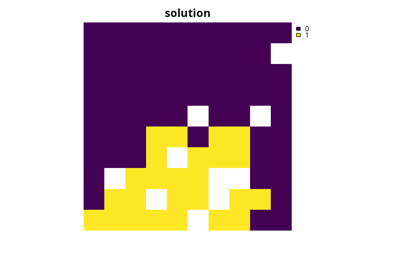
# create problem with maximum utility objective
p1 <-
  problem(sim_pu_raster, sim_features) %>%
  add_max_wtd_sum_objective(5000) %>%
  add_binary_decisions() %>%
  add_default_solver(gap = 0, verbose = FALSE)
#> ℹ `add_max_wtd_sum_objective()` has severe limitations - use with caution.

# solve problem
s1 <- solve(p1)

# plot solution
plot(s1, main = "solution", axes = FALSE)


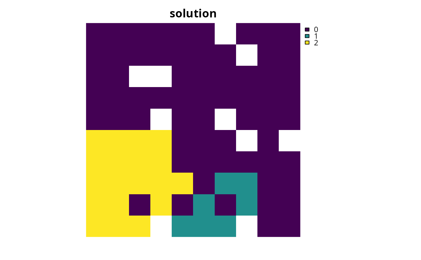
# create multi-zone problem with maximum utility objective that
# has a single budget for all zones
p2 <-
  problem(sim_zones_pu_raster, sim_zones_features) %>%
  add_max_wtd_sum_objective(5000) %>%
  add_binary_decisions() %>%
  add_default_solver(gap = 0, verbose = FALSE)
#> ℹ `add_max_wtd_sum_objective()` has severe limitations - use with caution.

# solve problem
s2 <- solve(p2)

# plot solution
plot(category_layer(s2), main = "solution", axes = FALSE)


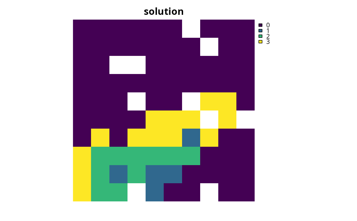
# create multi-zone problem with maximum utility objective that
# has separate budgets for each zone
p3 <-
  problem(sim_zones_pu_raster, sim_zones_features) %>%
  add_max_wtd_sum_objective(c(1000, 2000, 3000)) %>%
  add_binary_decisions() %>%
  add_default_solver(gap = 0, verbose = FALSE)
#> ℹ `add_max_wtd_sum_objective()` has severe limitations - use with caution.

# solve problem
s3 <- solve(p3)

# plot solution
plot(category_layer(s3), main = "solution", axes = FALSE)