Add penalties to a conservation planning problem to penalize
solutions that select planning units with higher cost values.
These penalties assume a linear trade-off between the cost and the primary
objective of the conservation planning problem (e.g.,
number of targets met for add_max_n_targets_met_objective().
Arguments
- x
problem()object.- penalty
numericvalue denoting the importance of not selecting planning units with high cost values. Higherpenaltyvalues can be used to obtain solutions that are strongly averse to selecting places with high cost values, and smallerpenaltyvalues can be used to obtain solutions that only avoid places with especially high cost. Note that negativepenaltyvalues can be used to obtain solutions that prefer places with high cost values. Additionally, if hasxhas multiple zones, thenpenaltymust have a value for each zone.
Value
An updated problem() object with the penalties added to it.
Details
This function penalizes solutions that have higher values according
to the sum of the cost values associated with each planning unit,
weighted by status of each planning unit in the solution.
Note that this function provided as a convenient alternative for
adding linear penalties (per add_linear_penalties()) to a problem().
Mathematical formulation
The cost penalties are implemented using the following
equations.
Let \(I\) denote the set of planning units
(indexed by \(i\)), \(Z\) the set of management zones (indexed by
\(z\)), and \(X_{iz}\) the decision variable for allocating
planning unit \(i\) to zone \(z\) (e.g., with binary
values indicating if each planning unit is allocated or not). Also, let
\(P_z\) represent the penalty scaling value for zones
\(z \in Z\) (per penalty), and
\(D_{iz}\) represent the cost data for allocating planning unit
\(i \in I\) to zones \(z \in Z\)
(per data in matrix format).
$$ \sum_{i}^{I} \sum_{z}^{Z} P_z \times D_{iz} \times X_{iz} $$
Note that when the problem objective is to maximize some measure of benefit and not minimize some measure of cost, the term \(P_z\) is replaced with \(-P_z\).
See also
Other functions for adding penalties:
add_asym_connectivity_penalties(),
add_boundary_penalties(),
add_connectivity_penalties(),
add_feature_weights(),
add_linear_penalties(),
add_neighbor_penalties()
Examples
# set seed for reproducibility
set.seed(600)
# load data
sim_complex_pu_raster <- get_sim_complex_pu_raster()
sim_complex_features <- get_sim_complex_features()
# create layer with 1s for all planning units
sim_ones_complex_raster <- (sim_complex_pu_raster * 0) + 1
# here we will formulate a multi-objective optimization problem
# that (i) minimizes the largest target shortfall for feature representation,
# (ii) minimizes the overall target shortfalls for feature representation,
# and (iii) minimizes the cost of the solution. since the
# first objective is to minimize the largest shortfall and the second
# objective is to minimize overall target shortfalls,
# this helps balance shortfalls among all features and better
# achieve complementarity. additionally, we will specify that
# (approximately) 30% of the study area should be selected (i.e., by
# specifying a budget for the upper threshold and a linear constraint for
# the lower threshold on the number of selected planning units).
# calculate budget based on 30% of the number of planning units
budget <-
0.3 * terra::global(sim_ones_complex_raster, "sum", na.rm = TRUE)[[1]]
# build multi-objective conservation planning problem
mp <-
multi_problem(
obj1 =
problem(sim_ones_complex_raster, sim_complex_features) %>%
add_min_largest_shortfall_objective(budget = budget) %>%
add_auto_targets("jung") %>%
# note that this constraint only needs to be specified once
add_cost_constraints(sense = ">=", budget = budget * 0.9) %>%
add_binary_decisions(),
obj2 =
problem(sim_ones_complex_raster, sim_complex_features) %>%
add_min_shortfall_objective(budget = budget) %>%
# note that we use the same targets for both obj1 and obj2
add_auto_targets("jung") %>%
add_binary_decisions(),
obj3 =
problem(sim_complex_pu_raster, sim_complex_pu_raster) %>%
add_min_penalties_objective() %>%
# note a value of 1 is here because only the costs minimized
add_cost_penalties(1) %>%
add_binary_decisions()
) %>%
add_default_solver(gap = 0.01, verbose = FALSE)
# to explore trade-offs between how well the feature targets
# are met and cost, we will generate a matrix of relative tolerance values
# for the hierarchical approach. note that the first column of this
# matrix will have only zeros to help promote balanced
# shortfalls across different features, and the second column
# will have non-zeros because we are interested in trade-offs between
# overall feature shortfalls and cost
rel_tol_matrix <- matrix(0, ncol = 2, nrow = 10)
rel_tol_matrix[, 2] <- seq(0, 0.5, length.out = nrow(rel_tol_matrix))
# display matrix
print(rel_tol_matrix)
#> [,1] [,2]
#> [1,] 0 0.00000000
#> [2,] 0 0.05555556
#> [3,] 0 0.11111111
#> [4,] 0 0.16666667
#> [5,] 0 0.22222222
#> [6,] 0 0.27777778
#> [7,] 0 0.33333333
#> [8,] 0 0.38888889
#> [9,] 0 0.44444444
#> [10,] 0 0.50000000
# add hierarchical approach to multi-objective problem
mp <-
mp %>%
add_hier_approach(rel_tol = rel_tol_matrix)
# generate solutions and remove duplicates
ms <- solve(mp, remove_duplicates = TRUE)
#> Generating solutions ■■■■ | 1/10 | 10% | ETA:32s
#> Generating solutions ■■■■■■■ | 2/10 | 20% | ETA:29s
#> Generating solutions ■■■■■■■■■■ | 3/10 | 30% | ETA:25s
#> Generating solutions ■■■■■■■■■■■■■ | 4/10 | 40% | ETA:21s
#> Generating solutions ■■■■■■■■■■■■■■■■ | 5/10 | 50% | ETA:18s
#> Generating solutions ■■■■■■■■■■■■■■■■■■■ | 6/10 | 60% | ETA:14s
#> Generating solutions ■■■■■■■■■■■■■■■■■■■■■■ | 7/10 | 70% | ETA:10s
#> Generating solutions ■■■■■■■■■■■■■■■■■■■■■■■■■ | 8/10 | 80% | ETA: 7s
#> Generating solutions ■■■■■■■■■■■■■■■■■■■■■■■■■■■■ | 9/10 | 90% | ETA: 3s
#> Generating solutions ■■■■■■■■■■■■■■■■■■■■■■■■■■■■■■■ | 10/10 | 100% | ETA: 0s
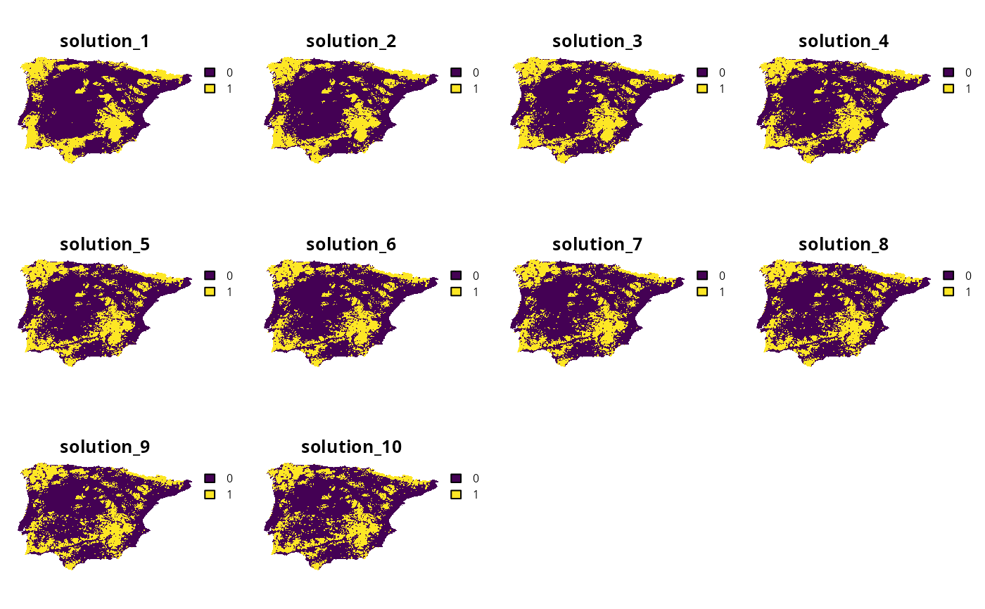
# plot the solutions
plot(terra::rast(ms), axes = FALSE)
 # extract objective values for the solutions
obj_matrix <- attributes(ms)$objective
# print the objective values
print(obj_matrix)
#> obj1 obj2 obj3
#> solution_1 0.5254115 17.44765 1027535.5
#> solution_2 0.5254618 18.41463 855765.4
#> solution_3 0.5254624 19.38561 771956.7
#> solution_4 0.5254624 20.35338 718990.5
#> solution_5 0.5254624 21.32408 680327.2
#> solution_6 0.5254624 22.29214 648289.1
#> solution_7 0.5254624 23.26140 620477.7
#> solution_8 0.5254624 24.22503 596998.6
#> solution_9 0.5254624 25.19655 576838.1
#> solution_10 0.5254624 26.16770 558808.8
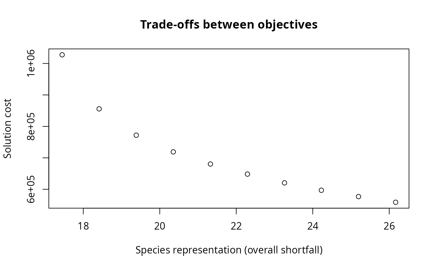
# plot the objectives values to visualize trade-offs
# (note that smaller values are better for both objectives)
plot(
obj_matrix[, 2:3],
main = "Trade-offs between objectives",
xlab = "Species representation (overall shortfall)",
ylab = "Solution cost"
)
# extract objective values for the solutions
obj_matrix <- attributes(ms)$objective
# print the objective values
print(obj_matrix)
#> obj1 obj2 obj3
#> solution_1 0.5254115 17.44765 1027535.5
#> solution_2 0.5254618 18.41463 855765.4
#> solution_3 0.5254624 19.38561 771956.7
#> solution_4 0.5254624 20.35338 718990.5
#> solution_5 0.5254624 21.32408 680327.2
#> solution_6 0.5254624 22.29214 648289.1
#> solution_7 0.5254624 23.26140 620477.7
#> solution_8 0.5254624 24.22503 596998.6
#> solution_9 0.5254624 25.19655 576838.1
#> solution_10 0.5254624 26.16770 558808.8
# plot the objectives values to visualize trade-offs
# (note that smaller values are better for both objectives)
plot(
obj_matrix[, 2:3],
main = "Trade-offs between objectives",
xlab = "Species representation (overall shortfall)",
ylab = "Solution cost"
)