Add maximum number of targets met objective
Source:R/add_max_n_targets_met.R
add_max_n_targets_met_objective.RdSet the objective of a conservation planning problem to
fulfill as many targets as possible, whilst ensuring that the cost of the
solution does not exceed a budget. Note that this objective does not
value the partial achievement of a given target—only whether or not
the target has been met. For this reason, we generally recommend using the
the minimum shortfall objective (add_min_shortfall_objective()
instead for budget-limited scenarios.
Arguments
- x
problem()object.- budget
numericvalue specifying the maximum expenditure permitted for the solution. Ifxhas multiple zones, thenbudgetcan be (i) a singlenumericvalue to specify an overall budget for the entire solution or (ii) anumericvector to specify a budget for each zone (separately) in the solution.
Details
The maximum number of targets met objective is an enhanced version of the
maximum coverage objective add_max_cover_objective() because
targets can be used to ensure that a certain amount of each feature is
required in order for them to be adequately represented (similar to the
minimum set objective (see add_min_set_objective()). This
objective finds the set of planning units that meets representation targets
for as many features as possible while staying within a fixed budget
(inspired by Cabeza and Moilanen 2001). Additionally, weights can be used
to favor the representation of certain features over other features (see
add_feature_weights()). If multiple solutions can meet the same
number of weighted targets while staying within budget, the cheapest
solution is returned.
Mathematical formulation
This objective can be expressed mathematically for a set of planning units (\(I\) indexed by \(i\)) and a set of features (\(J\) indexed by \(j\)) as:
$$\mathit{Maximize} \space \sum_{j = 1}^{J} y_j w_j \\ \mathit{subject \space to} \\ \sum_{i = 1}^{I} x_i r_{ij} \geq y_j t_j \forall j \in J \\ \sum_{i = 1}^{I} x_i c_i \leq B$$
Here, \(x_i\) is the decisions variable (e.g.,
specifying whether planning unit \(i\) has been selected (1) or not
(0)), \(r_{ij}\) is the amount of feature \(j\) in planning
unit \(i\), \(t_j\) is the representation target for feature
\(j\), \(y_j\) indicates if the solution has meet
the target \(t_j\) for feature \(j\), and \(w_j\) is the
weight for feature \(j\) (defaults to 1 for all features; see
add_feature_weights() to specify weights). Additionally,
\(B\) is the budget allocated for the solution, and \(c_i\) is the
cost of planning unit \(i\).
Notes
In previous versions (< 9.0.0), this function was called the
add_max_features_objective() and has since been renamed to
provide greater clarity. Additionally, it previously had extra
terms to help minimize the solution cost. Although these terms
have since been removed to reduce solve time,
this behavior can still be achieved by
building a multi-objective optimization problem and specifying the
first problem based on this objective function and the second
problem based on minimizing penalties (via add_min_penalties_objective())
with penalties set according to cost values
(via add_linear_penalties()).
References
Cabeza M and Moilanen A (2001) Design of reserve networks and the persistence of biodiversity. Trends in Ecology & Evolution, 16: 242–248.
See also
See objectives for an overview of all functions for adding objectives.
Also, see targets for an overview of all functions for adding targets, and
add_feature_weights() to specify weights for different features.
Other functions for adding objectives:
add_max_cover_objective(),
add_max_phylo_div_objective(),
add_max_phylo_end_objective(),
add_max_wtd_sum_objective(),
add_min_largest_shortfall_objective(),
add_min_penalties_objective(),
add_min_set_objective(),
add_min_shortfall_objective()
Examples
# load data
sim_pu_raster <- get_sim_pu_raster()
sim_features <- get_sim_features()
sim_zones_pu_raster <- get_sim_zones_pu_raster()
sim_zones_features <- get_sim_zones_features()
# create problem with maximum number of targets met objective
p1 <-
problem(sim_pu_raster, sim_features) %>%
add_max_n_targets_met_objective(1800) %>%
add_relative_targets(0.1) %>%
add_binary_decisions() %>%
add_default_solver(verbose = FALSE)
# solve problem
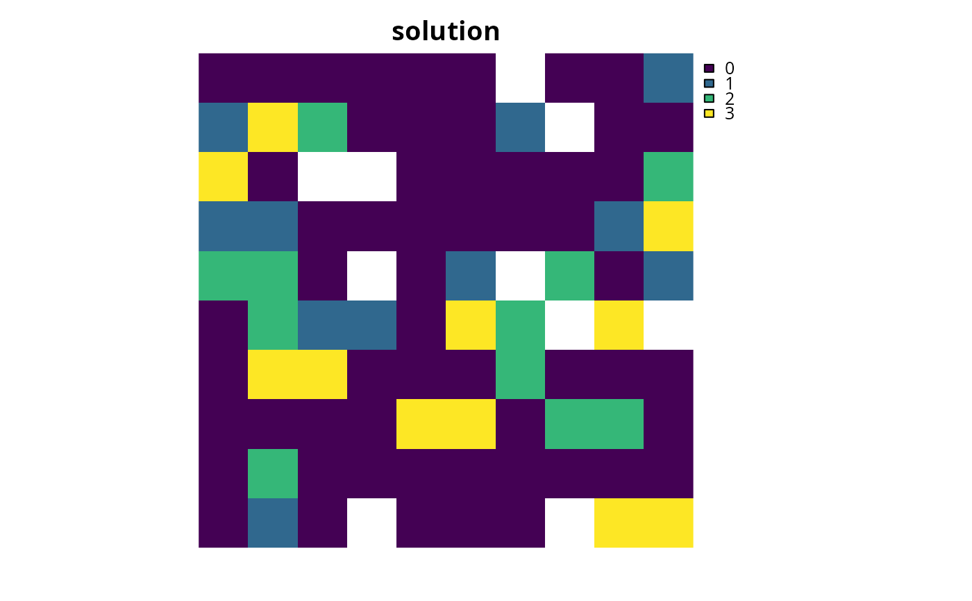
s1 <- solve(p1)
# plot solution
plot(s1, main = "solution", axes = FALSE)
 # create multi-zone problem with maximum number of targets met objective,
# 10% representation targets for each feature, and set
# a budget such that the total maximum expenditure in all zones
# cannot exceed 3000
p2 <-
problem(sim_zones_pu_raster, sim_zones_features) %>%
add_max_n_targets_met_objective(3000) %>%
add_relative_targets(matrix(0.1, ncol = 3, nrow = 5)) %>%
add_binary_decisions() %>%
add_default_solver(verbose = FALSE)
# solve problem
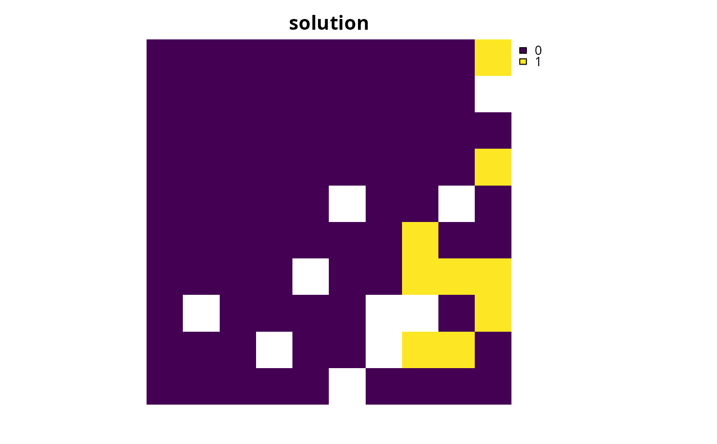
s2 <- solve(p2)
# plot solution
plot(category_layer(s2), main = "solution", axes = FALSE)
# create multi-zone problem with maximum number of targets met objective,
# 10% representation targets for each feature, and set
# a budget such that the total maximum expenditure in all zones
# cannot exceed 3000
p2 <-
problem(sim_zones_pu_raster, sim_zones_features) %>%
add_max_n_targets_met_objective(3000) %>%
add_relative_targets(matrix(0.1, ncol = 3, nrow = 5)) %>%
add_binary_decisions() %>%
add_default_solver(verbose = FALSE)
# solve problem
s2 <- solve(p2)
# plot solution
plot(category_layer(s2), main = "solution", axes = FALSE)
 # create multi-zone problem with maximum number of targets met objective,
# 10% representation targets for each feature, and set
# separate budgets for each management zone
p3 <-
problem(sim_zones_pu_raster, sim_zones_features) %>%
add_max_n_targets_met_objective(c(3000, 3000, 3000)) %>%
add_relative_targets(matrix(0.1, ncol = 3, nrow = 5)) %>%
add_binary_decisions() %>%
add_default_solver(verbose = FALSE)
# solve problem
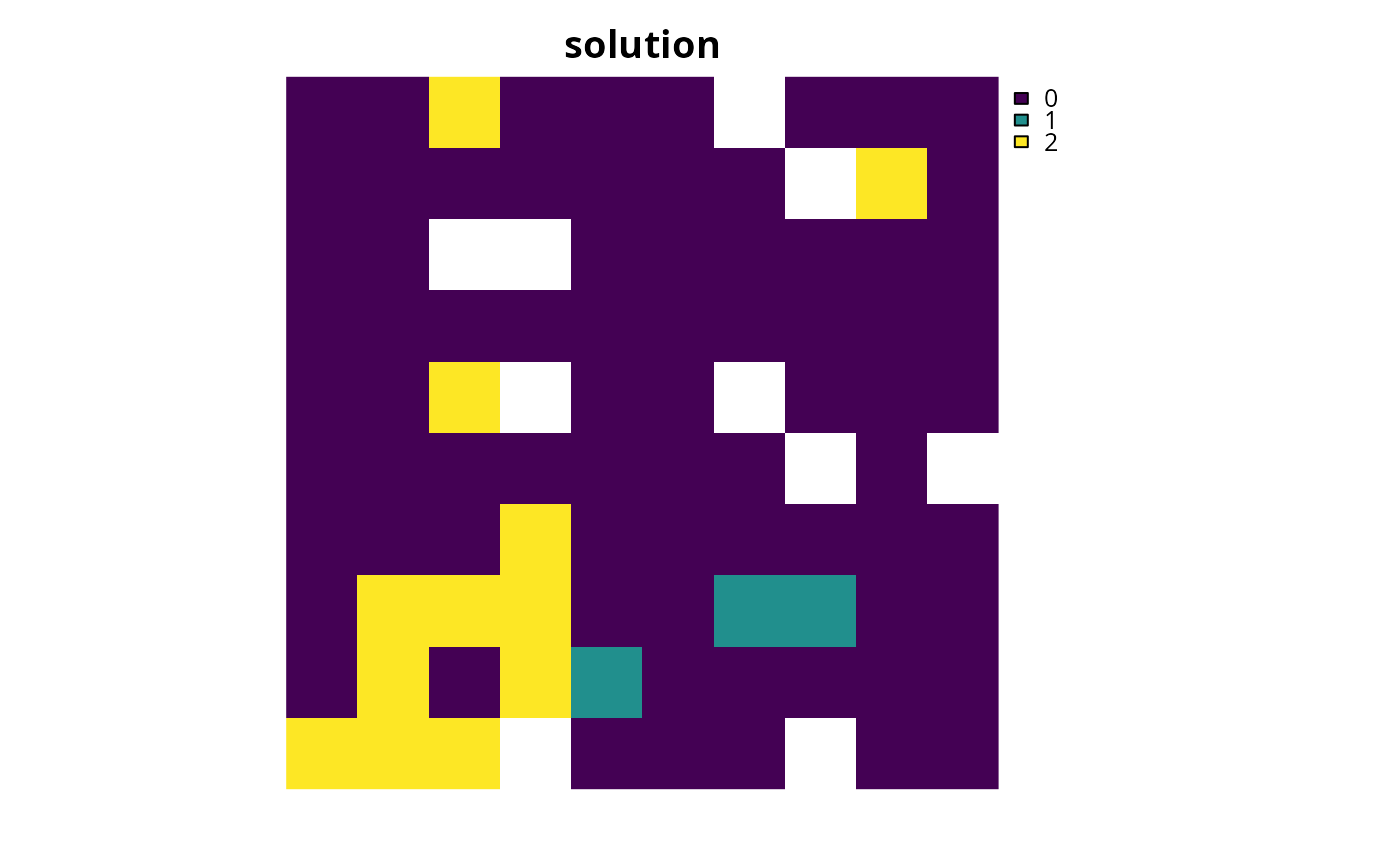
s3 <- solve(p3)
# plot solution
plot(category_layer(s3), main = "solution", axes = FALSE)
# create multi-zone problem with maximum number of targets met objective,
# 10% representation targets for each feature, and set
# separate budgets for each management zone
p3 <-
problem(sim_zones_pu_raster, sim_zones_features) %>%
add_max_n_targets_met_objective(c(3000, 3000, 3000)) %>%
add_relative_targets(matrix(0.1, ncol = 3, nrow = 5)) %>%
add_binary_decisions() %>%
add_default_solver(verbose = FALSE)
# solve problem
s3 <- solve(p3)
# plot solution
plot(category_layer(s3), main = "solution", axes = FALSE)