Add an approach

An approach can be added to a multi-objective conservation planning problem to specify the multi-objective optimization algorithm for generating solutions (López Jaimes et al. 2009).

Details

Multi-objective optimization approaches can be used to identify solutions that achieve multiple criteria (López Jaimes et al. 2009). For example, these approaches can help inform multi-use planning, where land use decisions must conserve biodiversity, meet food demands, and provide adequate housing supply (Neubert et al. 2025). These approaches can also be used to accommodate trade-offs between competing conservation objectives, such as representing multiple different conservation features (Deléglise et al. 2024) or minimizing multiple different cost datasets (Schuster et al. 2023). The following functions can be used to add an approach for multi-objective optimization to a multi-objective conservation planning multi_problem().

add_hier_approach(): Add an approach that involves solving each problem() in a multi_problem() object in a hierarchical (lexicographic) manner, wherein those associated with a higher priority order are solved before those with a lower priority order. Relative tolerance parameters can also be used to allow the optimization process to degrade objectives (in other words, allow for more wiggle room) so that subsequent (lower priority) objectives can be better achieved.
add_ref_point_approach(): Add an approach that involves using the reference point approach for multi-objective optimization. Briefly, this approach involves combining the objectives functions associated with each each problem() in a multi_problem() object into a single new objective, wherein reference point parameters are used to specify aspirational levels of achievement and weight parameters are used to specify the relative importance of each objective. To ensure that differences in scale among objective do not bias solutions, this approach also considers the best and worst possible objective values for each problem().
add_wtd_sum_approach(): Add an approach that involves combining the objective functions associated with each problem() in a multi_problem() object into a single new objective, wherein weights are used to specify the relative importance of each objective.

Note that although multi-objective approaches can be used to generate multiple solutions, they are conceptually different to methods for generating portfolios of solutions (see portfolios for details). This is because methods for generating solution portfolios identify multiple solutions that represent alternative spatial configurations for achieving the same particular objective (e.g., minimizing cost per add_min_set_objective()). Conversely, multi-objective approaches generate a single solution based on a set of parameters (e.g., weight or relative tolerance parameters) that specify trade-offs among multiple different objectives (e.g., minimizing cost per add_min_set_objective() and minimizing shortfalls in feature representation per add_min_shortfall_objective()). By specifying multiple sets of trade-off parameters, multi-objective approaches can be used to generate multiple solutions that represent different levels of compromise among the multiple objectives.

Recommended practices

In general, we recommend using the hierarchical approach (add_hier_approach()) for characterizing trade-offs between different objectives. Additionally, we recommend using the reference point approach to generate solutions that represent a balanced compromise among multiple objectives. Although the weighted sum approach (add_wtd_sum_approach()) is conceptually much easier to understand than the other approaches, it can be challenging to use in practice because it is sensitive to scaling issues— meaning that practitioners will often have to (i) consider a large number of combinations of weights to obtain a diverse set of solutions and (ii) perform multiple calibration procedures to manually identify weight parameter values that result in different solutions (Das and Dennis 1997).

References

Das I and Dennis JE (1997) A closer look at drawbacks of minimizing weighted sums of objectives for Pareto set generation in multicriteria optimization problems. Structural Optimization, 14: 63–69.

Deléglise H, Justeau-Allaire D, Mulligan M, Espinoza J-C, Isasi-Catalá E, Alvarez C, Condom T, and Palomo I (2024) Integrating multi-objective optimization and ecological connectivity to strengthen Peru's protected area system towards the 30*2030 target. Biological Conservation, 299: 110799.

López Jaimes A, Zapotecas Martínez S, and Coello Coello CA (2009) An introduction to multiobjective optimization techniques in Optimization in Polymer Processing. Eds Gaspar-Cunha A and Covas JA. Nova Science Publishers Inc, New York, United States.

Neubert S, McGowan J, Metcalfe K, Hanson JO, Buenafe KCV, Dabalà A, Dunn DC, Everett JD, Possingham HP, Stelzenmüller V, Estep A, Ervin J, and Richardson AJ (2025) Multiple-use spatial planning for sustainable development and conservation. Trends in Ecology and Evolution, 40: 1126–1142.

Schuster R, Buxton R, Hanson JO, Binley AD, Pittman J, Tulloch V, La Sorte FA, Roehrdanz PR, Verburg PH, Rodewald AD, Wilson S, Possingham HP, and Bennett JR (2022) Protected area planning to conserve biodiversity in an uncertain future. Conservation Biology, 37: e14048.

Examples

# in this example, we aim to identify a set of planning units that will
# not exceed a particular budget and meet objectives for
# (i) representing species that are important for ecosystem
# functioning (hereafter, keystone species) and (ii) representing species
# that have high social or cultural value (hereafter, iconic species)

# import data
con_cost <- get_sim_pu_raster()
keystone_spp <- get_sim_features()[[1:3]]
iconic_spp <- get_sim_features()[[4:5]]

# define a total conservation budget (30% of total cost)
budget <- terra::global(con_cost, "sum", na.rm = TRUE)[[1]] * 0.3

# now create multi-objective problem
mp <-
  multi_problem(
    keystone_obj =
      problem(con_cost, keystone_spp) %>%
      add_min_shortfall_objective(budget) %>%
      add_relative_targets(0.4) %>%
      add_binary_decisions(),
    iconic_obj =
      problem(con_cost, iconic_spp) %>%
      add_min_shortfall_objective(budget) %>%
      add_relative_targets(0.2) %>%
      add_binary_decisions()
  ) %>%
  add_default_solver(gap = 0, verbose = FALSE)

# create multi-problem with hierarchical approach,
# with settings to allow for 10% reduction in performance
# for the keystone objective to optimize the iconic objective
mp1 <-
 mp %>%
 add_hier_approach(rel_tol = 0.1, verbose = FALSE)

# create multi-problem with reference point approach,
# with settings identify a balanced compromise among objectives
mp2 <-
 mp %>%
 add_ref_point_approach(verbose = FALSE)

# create multi-problem with weighted sum approach,
# with weights to emphasize the keystone objective more than the
# iconic objective
mp3 <-
  mp %>%
  add_wtd_sum_approach(weights = c(0.9, 0.1), verbose = FALSE)

# solve problems
s <- c(solve(mp1), solve(mp2), solve (mp3))
names(s) <- c("hierarchical", "reference point", "weighted sum")

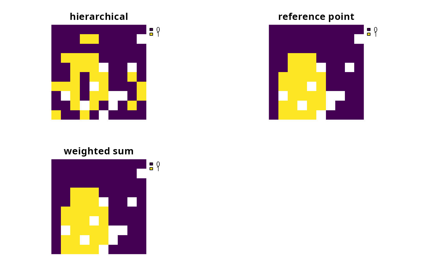
# plot solutions
plot(s, axes = FALSE)

Details

Recommended practices

References

See also

Examples